Category: number theory

Monstrous dessins 3

Published August 3, 2019 by lievenlb

A long while ago I promised to take you from the action by the modular group $\Gamma=PSL_2(\mathbb{Z})$ on the lattices at hyperdistance $n$ from the standard orthogonal laatice $L_1$ to the corresponding ‘monstrous’ Grothendieck dessin d’enfant.

Speaking of dessins d’enfant, let me point you to the latest intriguing paper by Yuri I. Manin and Matilde Marcolli, ArXived a few days ago Quantum Statistical Mechanics of the Absolute Galois Group, on how to build a quantum system for the absolute Galois group from dessins d’enfant (more on this, I promise, later).

Where were we?

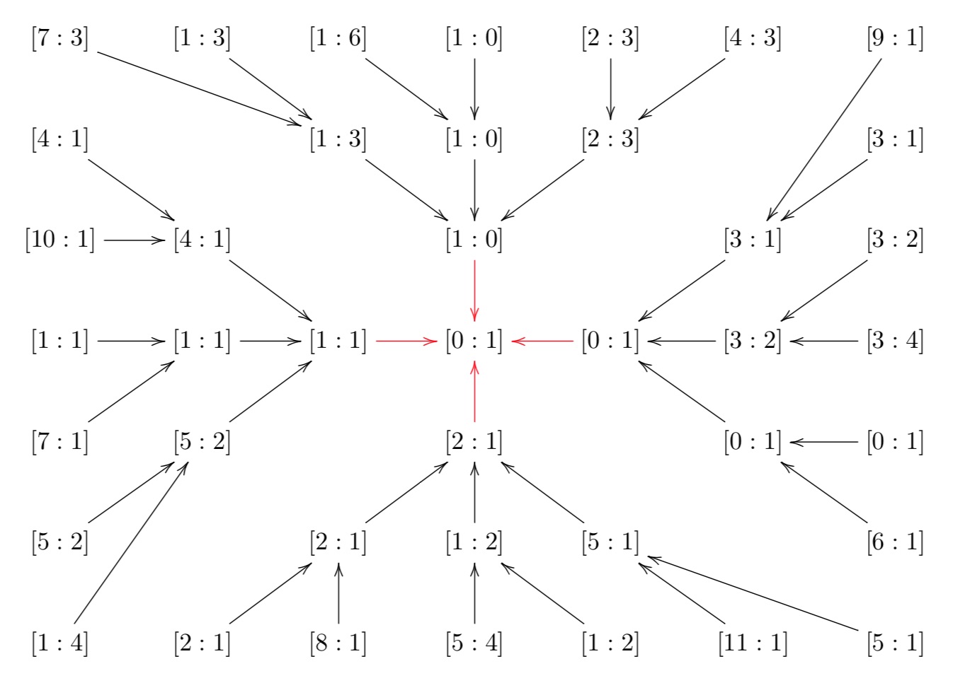
We’ve seen natural one-to-one correspondences between (a) points on the projective line over $\mathbb{Z}/n\mathbb{Z}$, (b) lattices at hyperdistance $n$ from $L_1$, and (c) coset classes of the congruence subgroup $\Gamma_0(n)$ in $\Gamma$.

How to get from there to a dessin d’enfant?

The short answer is: it’s all in Ravi S. Kulkarni’s paper, “An arithmetic-geometric method in the study of the subgroups of the modular group”, Amer. J. Math 113 (1991) 1053-1135.

It is a complete mystery to me why Tatitscheff, He and McKay don’t mention Kulkarni’s paper in “Cusps, congruence groups and monstrous dessins”. Because all they do (and much more) is in Kulkarni.

I’ve blogged about Kulkarni’s paper years ago:

– In the Dedekind tessalation it was all about assigning special polygons to subgroups of finite index of $\Gamma$.

– In Modular quilts and cuboid tree diagram it did go on assigning (multiple) cuboid trees to a (conjugacy class) of such finite index subgroup.

– In Hyperbolic Mathieu polygons the story continued on a finite-to-one connection between special hyperbolic polygons and cuboid trees.

– In Farey codes it was shown how to encode such polygons by a Farey-sequence.

– In Generators of modular subgroups it was shown how to get generators of the finite index subgroups from this Farey sequence.

The modular group is a free product
\[
\Gamma = C_2 \ast C_3 = \langle s,u~|~s^2=1=u^3 \rangle \]
with lifts of $s$ and $u$ to $SL_2(\mathbb{Z})$ given by the matrices
\[
S=\begin{bmatrix} 0 & -1 \\ 1 & 0 \end{bmatrix},~\qquad U= \begin{bmatrix} 0 & -1 \\ 1 & -1 \end{bmatrix} \]

As a result, any permutation representation of $\Gamma$ on a set $E$ can be represented by a $2$-coloured graph (with black and white vertices) and edges corresponding to the elements of the set $E$.

Each white vertex has two (or one) edges connected to it and every black vertex has three (or one). These edges are the elements of $E$ permuted by $s$ (for white vertices) and $u$ (for black ones), the order of the 3-cycle determined by going counterclockwise round the vertex.

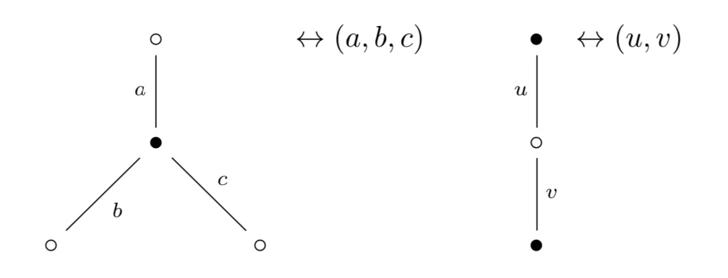
Clearly, if there’s just one edge connected to a vertex, it gives a fixed point (or 1-cycle) in the corresponding permutation.

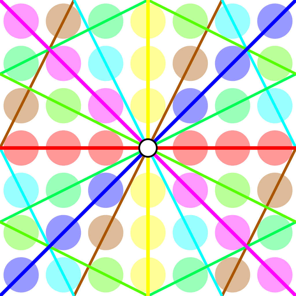
The ‘monstrous dessin’ for the congruence subgroup $\Gamma_0(n)$ is the picture one gets from the permutation $\Gamma$-action on the points of $\mathbb{P}^1(\mathbb{Z}/n \mathbb{Z})$, or equivalently, on the coset classes or on the lattices at hyperdistance $n$.

Kulkarni’s paper (or the blogposts above) tell you how to get at this picture starting from a fundamental domain of $\Gamma_0(n)$ acting on teh upper half-plane by Moebius transformations.

Sage gives a nice image of this fundamental domain via the command

FareySymbol(Gamma0(n)).fundamental_domain()

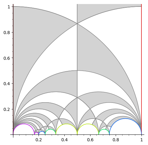
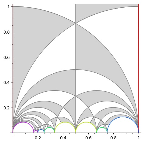
Here’s the image for $n=6$:

The boundary points (on the halflines through $0$ and $1$ and the $4$ half-circles need to be identified which is indicaed by matching colours. So the 2 halflines are identified as are the two blue (and green) half-circles (in opposite direction).

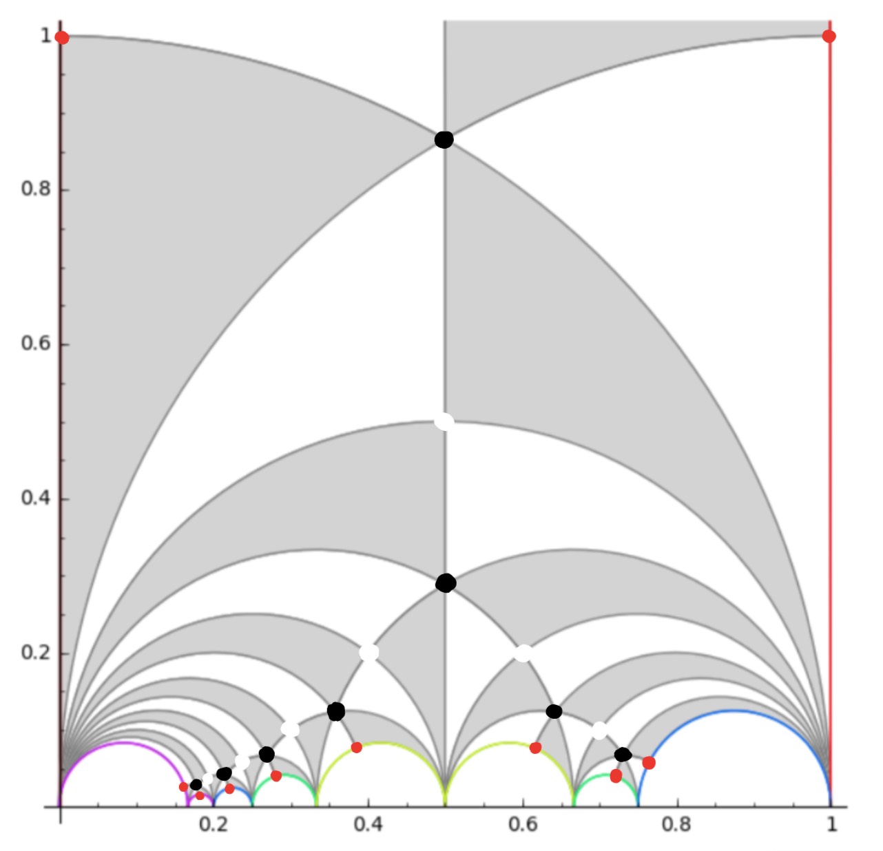
To get the dessin from this, let’s first look at the interior points. A white vertex is a point in the interior where two black and two white tiles meet, a black vertex corresponds to an interior points where three black and three white tiles meet.

Points on the boundary where tiles meet are coloured red, and after identification two of these reds give one white or black vertex. Here’s the intermediate picture

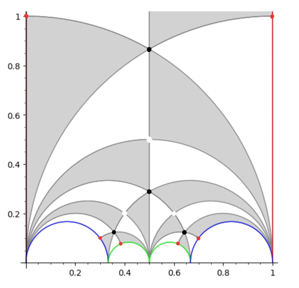
The two top red points are identified giving a white vertex as do the two reds on the blue half-circles and the two reds on the green half-circles, because after identification two black and two white tiles meet there.

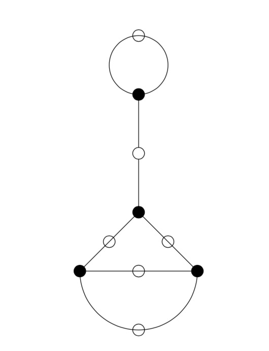
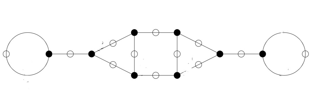
This then gives us the ‘monstrous’ modular dessin for $n=6$ of the Tatitscheff, He and McKay paper:

Let’s try a more difficult example: $n=12$. Sage gives us as fundamental domain

giving us the intermediate picture

and spotting the correct identifications, this gives us the ‘monstrous’ dessin for $\Gamma_0(12)$ from the THM-paper:

In general there are several of these 2-coloured graphs giving the same permutation representation, so the obtained ‘monstrous dessin’ depends on the choice of fundamental domain.

You’ll have noticed that the domain for $\Gamma_0(6)$ was symmetric, whereas the one Sage provides for $\Gamma_0(12)$ is not.

This is caused by Sage using the Farey-code
\[
\xymatrix{
0 \ar@{-}[r]_1 & \frac{1}{6} \ar@{-}[r]_1 & \frac{1}{5} \ar@{-}[r]_2 & \frac{1}{4} \ar@{-}[r]_3 & \frac{1}{3} \ar@{-}[r]_4 & \frac{1}{2} \ar@{-}[r]_4 & \frac{2}{3} \ar@{-}[r]_3 & \frac{3}{4} \ar@{-}[r]_2 & 1}
\]

One of the nice results from Kulkarni’s paper is that for any $n$ there is a symmetric Farey-code, giving a perfectly symmetric fundamental domain for $\Gamma_0(n)$. For $n=12$ this symmetric code is

\[
\xymatrix{
0 \ar@{-}[r]_1 & \frac{1}{6} \ar@{-}[r]_2 & \frac{1}{4} \ar@{-}[r]_3 & \frac{1}{3} \ar@{-}[r]_4 & \frac{1}{2} \ar@{-}[r]_4 & \frac{2}{3} \ar@{-}[r]_3 & \frac{3}{4} \ar@{-}[r]_2 & \frac{5}{6} \ar@{-}[r]_1 & 1}
\]

It would be nice to see whether using these symmetric Farey-codes gives other ‘monstrous dessins’ than in the THM-paper.

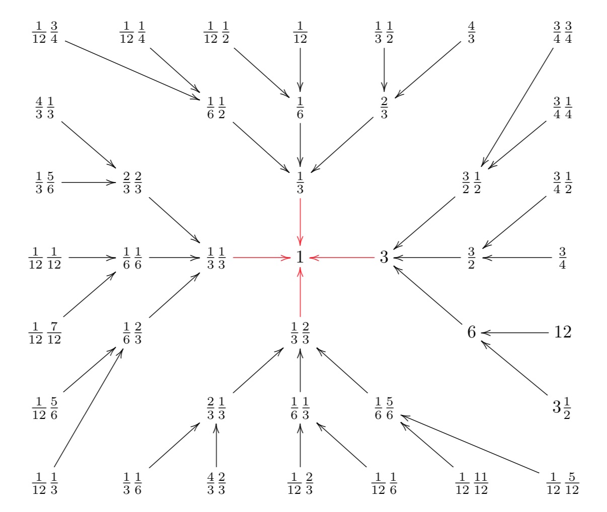
Remains to identify the edges in the dessin with the lattices at hyperdistance $n$ from $L_1$.

Using the tricks from the previous post it is quite easy to check that for any $n$ the monstrous dessin for $\Gamma_0(n)$ starts off with the lattices $L_{M,\frac{g}{h}} = M,\frac{g}{h}$ as below

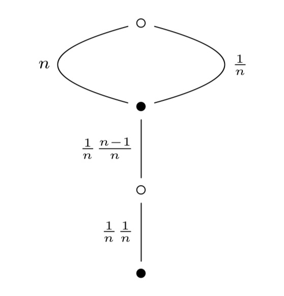
Let’s do a sample computation showing that the action of $s$ on $L_n$ gives $L_{\frac{1}{n}}$:

\[
L_n.s = \begin{bmatrix} n & 0 \\ 0 & 1 \end{bmatrix} \begin{bmatrix} 0 & -1 \\ 1 & 0 \end{bmatrix} = \begin{bmatrix} 0 & -n \\ 1 & 0 \end{bmatrix} \]

and then, as last time, to determine the class of the lattice spanned by the rows of this matrix we have to compute

\[
\begin{bmatrix} 0 & -1 \\ 1 & 0 \end{bmatrix} \begin{bmatrix} 0 & -n \\ 1 & 0 \end{bmatrix} = \begin{bmatrix} -1 & 0 \\ 0 & -n \end{bmatrix} \]

which is class $L_{\frac{1}{n}}$. And similarly for the other edges.

2 Comments

Monstrous dessins 2

Published July 24, 2019 by lievenlb

Let’s try to identify the $\Psi(n) = n \prod_{p|n}(1+\frac{1}{p})$ points of $\mathbb{P}^1(\mathbb{Z}/n \mathbb{Z})$ with the lattices $L_{M \frac{g}{h}}$ at hyperdistance $n$ from the standard lattice $L_1$ in Conway’s big picture.

Here are all $24=\Psi(12)$ lattices at hyperdistance $12$ from $L_1$ (the boundary lattices):

You can also see the $4 = \Psi(3)$ lattices at hyperdistance $3$ (those connected to $1$ with a red arrow) as well as the intermediate $12 = \Psi(6)$ lattices at hyperdistance $6$.

The vertices of Conway’s Big Picture are the projective classes of integral sublattices of the standard lattice $\mathbb{Z}^2=\mathbb{Z} e_1 \oplus \mathbb{Z} e_2$.

Let’s say our sublattice is generated by the integral vectors $v=(v_1,v_2)$ and $w=(w_1.w_2)$. How do we determine its class $L_{M,\frac{g}{h}}$ where $M \in \mathbb{Q}_+$ is a strictly positive rational number and $0 \leq \frac{g}{h} < 1$?

Here’s an example: the sublattice (the thick dots) is spanned by the vectors $v=(2,1)$ and $w=(1,4)$

Well, we try to find a basechange matrix in $SL_2(\mathbb{Z})$ such that the new 2nd base vector is of the form $(0,z)$. To do this take coprime $(c,d) \in \mathbb{Z}^2$ such that $cv_1+dw_1=0$ and complete with $(a,b)$ satisfying $ad-bc=1$ via Bezout to a matrix in $SL_2(\mathbb{Z})$ such that
\[
\begin{bmatrix} a & b \\ c & d \end{bmatrix} \begin{bmatrix} v_1 & v_2 \\ w_1 & w_2 \end{bmatrix} = \begin{bmatrix} x & y \\ 0 & z \end{bmatrix} \]
then the sublattice is of class $L_{\frac{x}{z},\frac{y}{z}~mod~1}$.

In the example, we have
\[
\begin{bmatrix} 0 & 1 \\ -1 & 2 \end{bmatrix} \begin{bmatrix} 2 & 1 \\ 1 & 4 \end{bmatrix} = \begin{bmatrix} 1 & 4 \\ 0 & 7 \end{bmatrix} \]
so this sublattice is of class $L_{\frac{1}{7},\frac{4}{7}}$.

Starting from a class $L_{M,\frac{g}{h}}$ it is easy to work out its hyperdistance from $L_1$: let $d$ be the smallest natural number making the corresponding matrix integral
\[
d. \begin{bmatrix} M & \frac{g}{h} \\ 0 & 1 \end{bmatrix} = \begin{bmatrix} u & v \\ 0 & w \end{bmatrix} \in M_2(\mathbb{Z}) \]
then $L_{M,\frac{g}{h}}$ is at hyperdistance $u . w$ from $L_1$.

Now that we know how to find the lattice class of any sublattice of $\mathbb{Z}^2$, let us assign a class to any point $[c:d]$ of $\mathbb{P}^1(\mathbb{Z}/n\mathbb{Z})$.

As $gcd(c,d)=1$, by Bezout we can find a integral matrix with determinant $1$
\[
S_{[c:d]} = \begin{bmatrix} a & b \\ c & d \end{bmatrix} \]
But then the matrix
\[
\begin{bmatrix} a.n & b.n \\ c & d \end{bmatrix} \]
has determinant $n$.

Working backwards we see that the class $L_{[c:d]}$ of the sublattice of $\mathbb{Z}^2$ spanned by the vectors $(a.n,b.n)$ and $(c,d)$ is of hyperdistance $n$ from $L_1$.

This is how the correspondence between points of $\mathbb{P}^1(\mathbb{Z}/n\mathbb{Z})$ and classes in Conway’s big picture at hyperdistance $n$ from $L_1$ works.

Let’s do an example. Take the point $[7:3] \in \mathbb{P}^1(\mathbb{Z}/12\mathbb{Z})$ (see last time), then
\[
\begin{bmatrix} -2 & -1 \\ 7 & 3 \end{bmatrix} \in SL_2(\mathbb{Z}) \]
so we have to determine the class of the sublattice spanned by $(-24,-12)$ and $(7,3)$. As before we have to compute
\[
\begin{bmatrix} -2 & -7 \\ 7 & 24 \end{bmatrix} \begin{bmatrix} -24 & -12 \\ 7 & 3 \end{bmatrix} = \begin{bmatrix} -1 & 3 \\ 0 & -12 \end{bmatrix} \]
giving us that the class $L_{[7:3]} = L_{\frac{1}{12}\frac{3}{4}}$ (remember that the second term must be taken $mod~1$).

If you do this for all points in $\mathbb{P}^1(\mathbb{Z}/12\mathbb{Z})$ (and $\mathbb{P}^1(\mathbb{Z}/6\mathbb{Z})$ and $\mathbb{P}^1(\mathbb{Z}/3 \mathbb{Z})$) you get this version of the picture we started with

You’ll spot that the preimages of a canonical coordinate of $\mathbb{P}^1(\mathbb{Z}/m\mathbb{Z})$ for $m | n$ are the very same coordinate together with ‘new’ canonical coordinates in $\mathbb{P}^1(\mathbb{Z}/n\mathbb{Z})$.

To see that this correspondence is one-to-one and that the index of the congruence subgroup
\[
\Gamma_0(n) = \{ \begin{bmatrix} p & q \\ r & s \end{bmatrix}~|~n|r~\text{and}~ps-qr=1 \} \]
in the full modular group $\Gamma = PSL_2(\mathbb{Z})$ is equal to $\Psi(n)$ it is useful to consider the action of $PGL_2(\mathbb{Q})^+$ on the right on the classes of lattices.

The stabilizer of $L_1$ is the full modular group $\Gamma$ and the stabilizer of any class is a suitable conjugate of $\Gamma$. For example, for the class $L_n$ (that is, of the sublattice spanned by $(n,0)$ and $(0,1)$, which is of hyperdistance $n$ from $L_1$) this stabilizer is
\[
Stab(L_n) = \{ \begin{bmatrix} a & \frac{b}{n} \\ c.n & d \end{bmatrix}~|~ad-bc = 1 \} \]
and a very useful observation is that
\[
Stab(L_1) \cap Stab(L_n) = \Gamma_0(n) \]
This is the way Conway likes us to think about the congruence subgroup $\Gamma_0(n)$: it is the joint stabilizer of the classes $L_1$ and $L_n$ (as well as all classes in the ‘thread’ $L_m$ with $m | n$).

On the other hand, $\Gamma$ acts by rotations on the big picture: it only fixes $L_1$ and maps a class to another one of the same hyperdistance from $L_1$.The index of $\Gamma_0(n)$ in $\Gamma$ is then the number of classes at hyperdistance $n$.

To see that this number is $\Psi(n)$, first check that the classes at hyperdistance $p^k$ for $p$ a prime number and for all $k$ for the $p+1$ free valent tree with root $L_1$, so there are exactly $p^{k-1}(p+1)$ classes as hyperdistance $p^k$.

To get from this that the number of hyperdistance $n$ classes is indeed $\Psi(n) = \prod_{p|n}p^{v_p(n)-1}(p+1)$ we have to use the prime- factorisation of the hyperdistance (see this post).

The fundamental domain for the action of $\Gamma_0(12)$ by Moebius tranfos on the upper half plane must then consist of $48=2 \Psi(12)$ black or white hyperbolic triangles

Next time we’ll see how to deduce the ‘monstrous’ Grothendieck dessin d’enfant for $\Gamma_0(12)$ from it

Monstrous dessins 1

Published July 22, 2019 by lievenlb

Dedekind’s Psi-function $\Psi(n)= n \prod_{p |n}(1 + \frac{1}{p})$ pops up in a number of topics:

$\Psi(n)$ is the index of the congruence subgroup $\Gamma_0(n)$ in the modular group $\Gamma=PSL_2(\mathbb{Z})$,
$\Psi(n)$ is the number of points in the projective line $\mathbb{P}^1(\mathbb{Z}/n\mathbb{Z})$,
$\Psi(n)$ is the number of classes of $2$-dimensional lattices $L_{M \frac{g}{h}}$ at hyperdistance $n$ in Conway’s big picture from the standard lattice $L_1$,
$\Psi(n)$ is the number of admissible maximal commuting sets of operators in the Pauli group of a single qudit.

The first and third interpretation have obvious connections with Monstrous Moonshine.

Conway’s big picture originated from the desire to better understand the Moonshine groups, and Ogg’s Jack Daniels problem
asks for a conceptual interpretation of the fact that the prime numbers such that $\Gamma_0(p)^+$ is a genus zero group are exactly the prime divisors of the order of the Monster simple group.

Here’s a nice talk by Ken Ono : Can’t you just feel the Moonshine?

For this reason it might be worthwhile to make the connection between these two concepts and the number of points of $\mathbb{P}^1(\mathbb{Z}/n\mathbb{Z})$ as explicit as possible.

Surely all of this is classical, but it is nicely summarised in the paper by Tatitscheff, He and McKay “Cusps, congruence groups and monstrous dessins”.

The ‘monstrous dessins’ from their title refers to the fact that the lattices $L_{M \frac{g}{h}}$ at hyperdistance $n$ from $L_1$ are permuted by the action of the modular groups and so determine a Grothendieck’s dessin d’enfant. In this paper they describe the dessins corresponding to the $15$ genus zero congruence subgroups $\Gamma_0(n)$, that is when $n=1,2,3,4,5,6,7,8,9,10,12,13,16,18$ or $25$.

Here’s the ‘monstrous dessin’ for $\Gamma_0(6)$

But, one can compute these dessins for arbitrary $n$, describing the ripples in Conway’s big picture, and try to figure out whether they are consistent with the Riemann hypothesis.

We will get there eventually, but let’s start at an easy pace and try to describe the points of the projective line $\mathbb{P}^1(\mathbb{Z}/n \mathbb{Z})$.

Over a field $k$ the points of $\mathbb{P}^1(k)$ correspond to the lines through the origin in the affine plane $\mathbb{A}^2(k)$ and they can represented by projective coordinates $[a:b]$ which are equivalence classes of couples $(a,b) \in k^2- \{ (0,0) \}$ under scalar multiplication with non-zero elements in $k$, so with points $[a:1]$ for all $a \in k$ together with the point at infinity $[1:0]$. When $n=p$ is a prime number we have $\# \mathbb{P}^1(\mathbb{Z}/p\mathbb{Z}) = p+1$. Here are the $8$ lines through the origin in $\mathbb{A}^2(\mathbb{Z}/7\mathbb{Z})$

Over an arbitrary (commutative) ring $R$ the points of $\mathbb{P}^1(R)$ again represent equivalence classes, this time of pairs
\[
(a,b) \in R^2~:~aR+bR=R \]
with respect to scalar multiplication by units in $R$, that is
\[
(a,b) \sim (c,d)~\quad~\text{iff}~\qquad \exists \lambda \in R^*~:~a=\lambda c, b = \lambda d \]
For $\mathbb{P}^1(\mathbb{Z}/n \mathbb{Z})$ we have to find all pairs of integers $(a,b) \in \mathbb{Z}^2$ with $0 \leq a,b < n$ with $gcd(a,b)=1$ and use Cremona’s trick to test for equivalence:
\[
(a,b) = (c,d) \in \mathbb{P}^1(\mathbb{Z}/n \mathbb{Z})~\quad \text{iff}~\quad ad-bc \equiv 0~mod~n \]
The problem is to find a canonical representative in each class in an efficient way because this is used a huge number of times in working with modular symbols.

Perhaps the best algorithm, for large $n$, is sketched in pages 145-146 of Bill Stein’s Modular forms: a computational approach.

For small $n$ the algorithm in $\S 1.3$ in the Tatitscheff, He and McKay paper suffices:

Consider the action of $(\mathbb{Z}/n\mathbb{Z})^*$ on $\{ 0,1,…,n-1 \}=\mathbb{Z}/n\mathbb{Z}$ and let $D$ be the set of the smallest elements in each orbit,
For each $d \in D$ compute the stabilizer subgroup $G_d$ for this action and let $C_d$ be the set of smallest elements in each $G_d$-orbit on the set of all elements in $\mathbb{Z}/n \mathbb{Z}$ coprime with $d$,
Then $\mathbb{P}^1(\mathbb{Z}/n\mathbb{Z})= \{ [c:d]~|~d \in D, c \in C_d \}$.

Let’s work this out for $n=12$ which will be our running example (the smallest non-squarefree non-primepower):

$(\mathbb{Z}/12\mathbb{Z})^* = \{ 1,5,7,11 \} \simeq C_2 \times C_2$,
The orbits on $\{ 0,1,…,11 \}$ are
\[
\{ 0 \}, \{ 1,5,7,11 \}, \{ 2,10 \}, \{ 3,9 \}, \{ 4,8 \}, \{ 6 \} \]
and $D=\{ 0,1,2,3,4,6 \}$,
$G_0 = C_2 \times C_2$, $G_1 = \{ 1 \}$, $G_2 = \{ 1,7 \}$, $G_3 = \{ 1,5 \}$, $G_4=\{ 1,7 \}$ and $G_6=C_2 \times C_2$,
$1$ is the only number coprime with $0$, giving us $[1:0]$,
$\{ 0,1,…,11 \}$ are all coprime with $1$, and we have trivial stabilizer, giving us the points $[0:1],[1:1],…,[11:1]$,
$\{ 1,3,5,7,9,11 \}$ are coprime with $2$ and under the action of $\{ 1,7 \}$ they split into the orbits
\[
\{ 1,7 \},~\{ 3,9 \},~\{ 5,11 \} \]
giving us the points $[1:2],[3:2]$ and $[5:2]$,
$\{ 1,2,4,5,7,8,10,11 \}$ are coprime with $3$, the action of $\{ 1,5 \}$ gives us the orbits
\[
\{ 1,5 \},~\{ 2,10 \},~\{ 4,8 \},~\{ 7,11 \} \]
and additional points $[1:3],[2:3],[4:3]$ and $[7:3]$,
$\{ 1,3,5,7,9,11 \}$ are coprime with $4$ and under the action of $\{ 1,7 \}$ we get orbits
\[
\{ 1,7 \},~\{ 3,9 \},~\{ 5,11 \} \]
and points $[1:4],[3:4]$ and $[5,4]$,
Finally, $\{ 1,5,7,11 \}$ are the only coprimes with $6$ and they form a single orbit under $C_2 \times C_2$ giving us just one additional point $[1:6]$.

This gives us all $24= \Psi(12)$ points of $\mathbb{P}^1(\mathbb{Z}/12 \mathbb{Z})$ (strangely, op page 43 of the T-H-M paper they use different representants).

One way to see that $\# \mathbb{P}^1(\mathbb{Z}/n \mathbb{Z}) = \Psi(n)$ comes from a consequence of the Chinese Remainder Theorem that for the prime factorization $n = p_1^{e_1} … p_k^{e_k}$ we have
\[
\mathbb{P}^1(\mathbb{Z}/n \mathbb{Z}) = \mathbb{P}^1(\mathbb{Z}/p_1^{e_1} \mathbb{Z}) \times … \times \mathbb{P}^1(\mathbb{Z}/p_k^{e_k} \mathbb{Z}) \]
and for a prime power $p^k$ we have canonical representants for $\mathbb{P}^1(\mathbb{Z}/p^k \mathbb{Z})$
\[
[a:1]~\text{for}~a=0,1,…,p^k-1~\quad \text{and} \quad [1:b]~\text{for}~b=0,p,2p,3p,…,p^k-p \]
which shows that $\# \mathbb{P}^1(\mathbb{Z}/p^k \mathbb{Z}) = (p+1)p^{k-1}= \Psi(p^k)$.

Next time, we’ll connect $\mathbb{P}^1(\mathbb{Z}/n \mathbb{Z})$ to Conway’s big picture and the congruence subgroup $\Gamma_0(n)$.