A Belyi-extender (or dessinflateur) $\beta$ of degree $d$ is a quotient of two polynomials with rational coefficients
\[
\beta(t) = \frac{f(t)}{g(t)} \]
with the special properties that for each complex number $c$ the polynomial equation of degree $d$ in $t$
\[
f(t)-c g(t)=0 \]
has $d$ distinct solutions, except perhaps for $c=0$ or $c=1$, and, in addition, we have that
\[
\beta(0),\beta(1),\beta(\infty) \in \{ 0,1,\infty \} \]
Let’s take for instance the power maps $\beta_n(t)=t^n$.
For every $c$ the degree $n$ polynomial $t^n – c = 0$ has exactly $n$ distinct solutions, except for $c=0$, when there is just one. And, clearly we have that $0^n=0$, $1^n=1$ and $\infty^n=\infty$. So, $\beta_n$ is a Belyi-extender of degree $n$.
A cute observation being that if $\beta$ is a Belyi-extender of degree $d$, and $\beta’$ is an extender of degree $d’$, then $\beta \circ \beta’$ is again a Belyi-extender, this time of degree $d.d’$.
That is, Belyi-extenders form a monoid under composition!
In our example, $\beta_n \circ \beta_m = \beta_{n.m}$. So, the power-maps are a sub-monoid of the Belyi-extenders, isomorphic to the multiplicative monoid $\mathbb{N}_{\times}$ of strictly positive natural numbers.

In their paper Quantum statistical mechanics of the absolute Galois group, Yuri I. Manin and Matilde Marcolli say they use the full monoid of Belyi-extenders to act on all Grothendieck’s dessins d’enfant.
But, they attach properties to these Belyi-extenders which they don’t have, in general. That’s fine, as they foresee in Remark 2.21 of their paper that the construction works equally well for any suitable sub-monoid, as long as this sub-monoid contains all power-map exenders.
I’m trying to figure out what the maximal mystery sub-monoid of extenders is satisfying all the properties they need for their proofs.
But first, let us see what Belyi-extenders have to do with dessins d’enfant.

In his user-friendlier period, Grothendieck told us how to draw a picture, which he called a dessin d’enfant, of an extender $\beta(t) = \frac{f(t)}{g(t)}$ of degree $d$:
Look at all complex solutions of $f(t)=0$ and label them with a black dot (and add a black dot at $\infty$ if $\beta(\infty)=0$). Now, look at all complex solutions of $f(t)-g(t)=0$ and label them with a white dot (and add a white dot at $\infty$ if $\beta(\infty)=1$).
Now comes the fun part.
Because $\beta$ has exactly $d$ pre-images for all real numbers $\lambda$ in the open interval $(0,1)$ (and $\beta$ is continuous), we can connect the black dots with the white dots by $d$ edges (the pre-images of the open interval $(0,1)$), giving us a $2$-coloured graph.
For the power-maps $\beta_n(t)=t^n$, we have just one black dot at $0$ (being the only solution of $t^n=0$), and $n$ white dots at the $n$-th roots of unity (the solutions of $x^n-1=0$). Any $\lambda \in (0,1)$ has as its $n$ pre-images the numbers $\zeta_i.\sqrt[n]{\lambda}$ with $\zeta_i$ an $n$-th root of unity, so we get here as picture an $n$-star. Here for $n=5$:
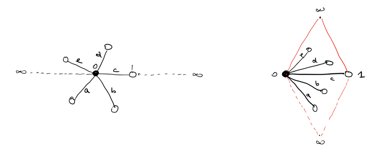
This dessin should be viewed on the 2-sphere, with the antipodal point of $0$ being $\infty$, so projecting from $\infty$ gives a homeomorphism between the 2-sphere and $\mathbb{C} \cup \{ \infty \}$.
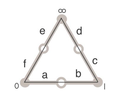
To get all information of the dessin (including possible dots at infinity) it is best to slice the sphere open along the real segments $(\infty,0)$ and $(1,\infty)$ and flatten it to form a ‘diamond’ with the upper triangle corresponding to the closed upper semisphere and the lower triangle to the open lower semisphere.
In the picture above, the right hand side is the dessin drawn in the diamond, and this representation will be important when we come to the action of extenders on more general Grothendieck dessins d’enfant.
Okay, let’s try to get some information about the monoid $\mathcal{E}$ of all Belyi-extenders.
What are its invertible elements?
Well, we’ve seen that the degree of a composition of two extenders is the product of their degrees, so invertible elements must have degree $1$, so are automorphisms of $\mathbb{P}^1_{\mathbb{C}} – \{ 0,1,\infty \} = S^2-\{ 0,1,\infty \}$ permuting the set $\{ 0,1,\infty \}$.
They form the symmetric group $S_3$ on $3$-letters and correspond to the Belyi-extenders
\[
t,~1-t,~\frac{1}{t},~\frac{1}{1-t},~\frac{t-1}{t},~\frac{t}{t-1} \]
You can compose these units with an extender to get anther extender of the same degree where the roles of $0,1$ and $\infty$ are changed.
For example, if you want to colour all your white dots black and the black dots white, you compose with the unit $1-t$.
Manin and Marcolli use this and claim that you can transform any extender $\eta$ to an extender $\gamma$ by composing with a unit, such that $\gamma(0)=0, \gamma(1)=1$ and $\gamma(\infty)=\infty$.
That’s fine as long as your original extender $\eta$ maps $\{ 0,1,\infty \}$ onto $\{ 0,1,\infty \}$, but usually a Belyi-extender only maps into $\{ 0,1,\infty \}$.
Here are some extenders of degree three (taken from Melanie Wood’s paper Belyi-extending maps and the Galois action on dessins d’enfants):
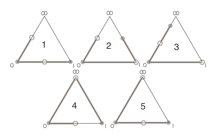
with dessin $5$ corresponding to the Belyi-extender
\[
\beta(t) = \frac{t^2(t-1)}{(t-\frac{4}{3})^3} \]
with $\beta(0)=0=\beta(1)$ and $\beta(\infty) = 1$.
So, a first property of the mystery Manin-Marcolli monoid $\mathcal{E}_{MMM}$ must surely be that all its elements $\gamma(t)$ map $\{ 0,1,\infty \}$ onto $\{ 0,1,\infty \}$, for they use this property a number of times, for instance to construct a monoid map
\[
\mathcal{E}_{MMM} \rightarrow M_2(\mathbb{Z})^+ \qquad \gamma \mapsto \begin{bmatrix} d & m-1 \\ 0 & 1 \end{bmatrix} \]
where $d$ is the degree of $\gamma$ and $m$ is the number of black dots in the dessin (or white dots for that matter).
Further, they seem to believe that the dessin of any Belyi-extender must be a 2-coloured tree.
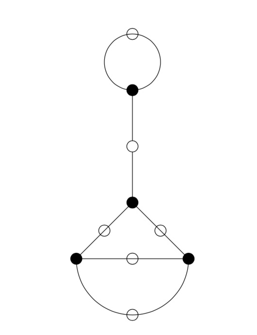
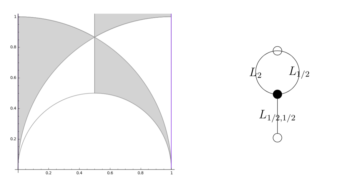
Already last time we’ve encountered a Belyi-extender $\zeta(t) = \frac{27 t^2(t-1)^2}{4(t^2-t+1)^3}$ with dessin
But then, you may argue, this extender sends all of $0,1$ and $\infty$ to $0$, so it cannot belong to $\mathcal{E}_{MMM}$.
Here’s a trick to construct Belyi-extenders from Belyi-maps $\beta : \mathbb{P}^1 \rightarrow \mathbb{P}^1$, defined over $\mathbb{Q}$ and having the property that there are rational points in the fibers over $0,1$ and $\infty$.
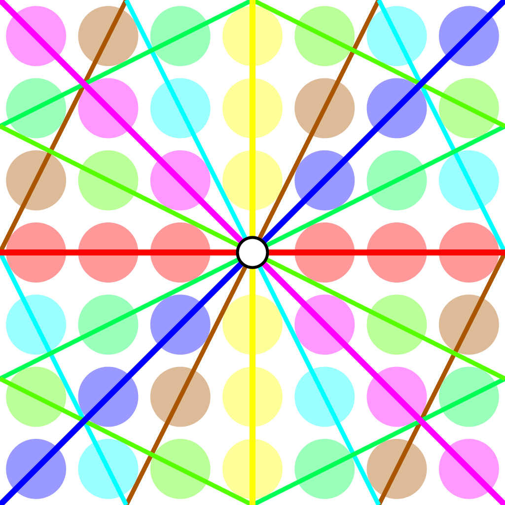
Let’s take an example, the ‘monstrous dessin’ corresponding to the congruence subgroup $\Gamma_0(2)$
with map $\beta(t) = \frac{(t+256)^3}{1728 t^2}$.
As it stands, $\beta$ is not a Belyi-extender because it does not map $1$ into $\{ 0,1,\infty \}$. But we have that
\[
-256 \in \beta^{-1}(0),~\infty \in \beta^{-1}(\infty),~\text{and}~512,-64 \in \beta^{-1}(1) \]
(the last one follows from $(t+256)^2-1728 t^3=(t-512)^2(t+64)$).
We can now pre-compose $\beta$ with the automorphism (defined over $\mathbb{Q}$) sending $0$ to $-256$, $1$ to $-64$ and fixing $\infty$ to get a Belyi-extender
\[
\gamma(t) = \frac{(192t)^3}{1728(192t-256)^2} \]
which maps $\gamma(0)=0,~\gamma(1)=1$ and $\gamma(\infty)=\infty$ (so belongs to $\mathcal{E}_{MMM}$) with the same dessin, which is not a tree,
That is, $\mathcal{E}_{MMM}$ can at best consist only of those Belyi-extenders $\gamma(t)$ that map $\{ 0,1,\infty \}$ onto $\{ 0,1,\infty \}$ and such that their dessin is a tree.
Let me stop, for now, by asking for a reference (or counterexample) to perhaps the most startling claim in the Manin-Marcolli paper, namely that any 2-coloured tree can be realised as the dessin of a Belyi-extender!