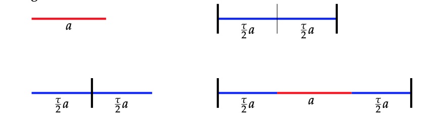
A Conway musical sequence is an infinite word in $L$ and $S$, containing no two consecutive $S$’s nor three consecutive $L$’s, such that all its inflations remain musical sequences.
We’ve seen that such musical sequences encode an aperiodic tiling of the line in short ($S$) and long ($L$) intervals, and that such tilings are all finite locally isomorphic.
But, apart from the middle $C$-sequences (the one-dimensional cartwheel tilings) we gave no examples of such tilings (or musical sequences). Let’s remedy this!
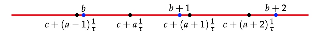
Take any real number $c$ as long as it is not an integral combination of $1$ and $\tfrac{1}{\tau}$ (with $\tau$ the golden ratio) and assign to any integer $a \in \mathbb{Z}$ a tile
\[
P_c(a) = \begin{cases} S \\ L \end{cases} ~\text{iff}~\lceil c+(a+1)\frac{1}{\tau} \rceil – \lceil c+a \frac{1}{\tau} \rceil = \begin{cases} 0 \\ 1 \end{cases} \]
(instead of ceilings we might have taken floors, because of the restriction on $c$).
With a little bit of work we see that the deflated word determined by $P_c$ is again of this type, more precisely $def(P_c) = P_{-(c-\lfloor c \rfloor)\frac{1}{\tau}}$. But then it also follows that inflated words are of this type, meaning that all $P_c$ define a musical sequence.
Let’s just check that these sequences satisfy the gluing restrictions. If there is no integer between $c+a\tfrac{1}{\tau}$ and $c+(a+1)\tfrac{1}{\tau}$, because $2 \tfrac{1}{\tau} \approx 1.236$ there must be an interval in the preceding and the following $\tfrac{1}{\tau}$-interval, showing that an $S$ in the sequence has an $L$ on its left and right, so there are no two consecutive $S$’s in the sequences.

Similarly, if two consecutive $\tfrac{1}{\tau}$-intervals have an integer in them, the next interval cannot contain an integer as $3 \tfrac{1}{\tau} \approx 1.854 < 2$.
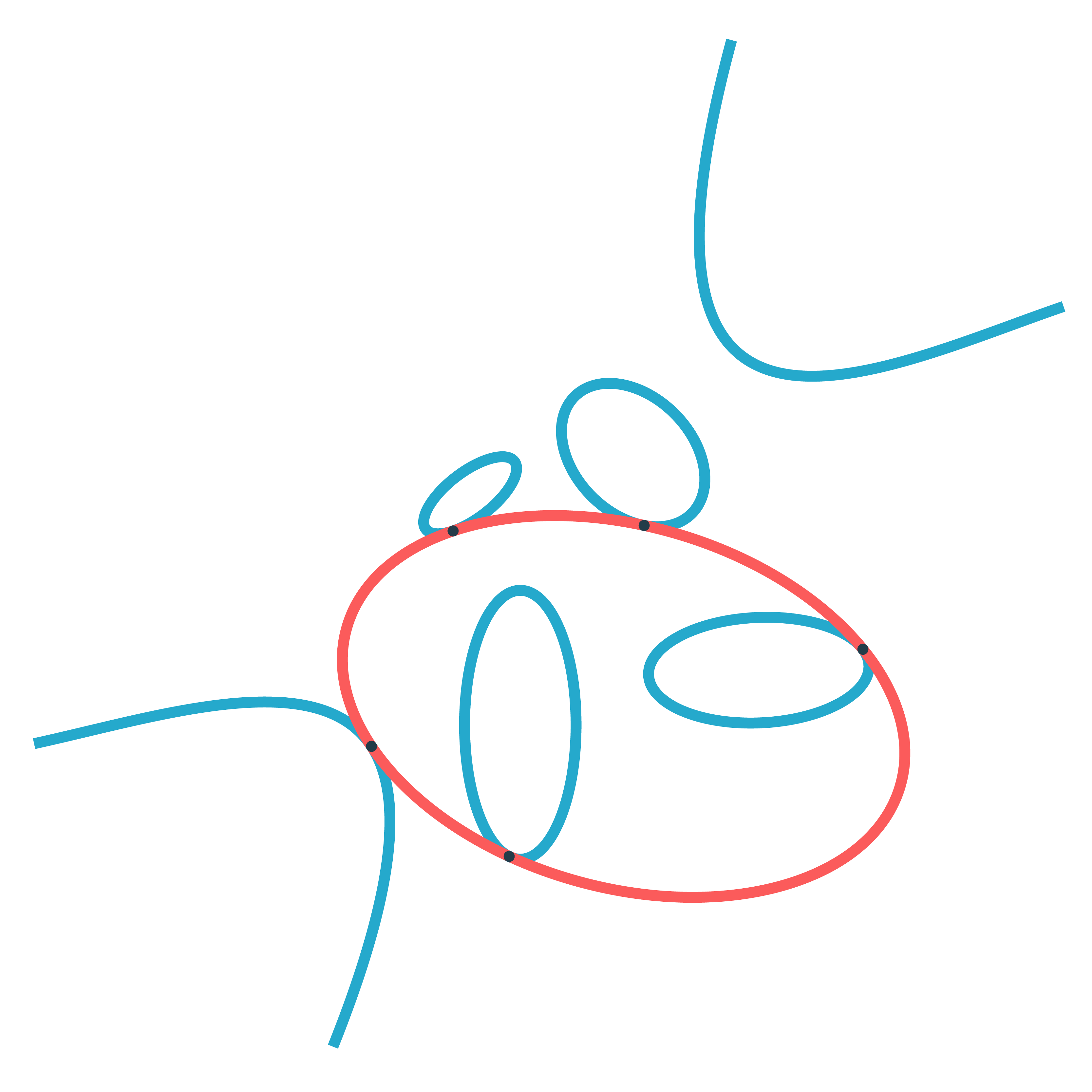
Now we come to the essential point: these sequences can be obtained by the cut-and-project method.
Take the line $L$ through the origin with slope $\tfrac{1}{\tau}$ and $L^{\perp}$ the line perpendicular it.
Consider the unit square $H$ and $H_{\vec{\gamma}}=H + \vec{\gamma}$ its translation under a shift vector $\vec{\gamma}=(\gamma_x,\gamma_y)$ and let $\pi$ (or $\pi^{\perp}$) be the orthogonal projection of the plane onto $L$ (or onto $L^{\perp}$). One quickly computes that
\[
\pi(a,b) = (\frac{\tau^2 a + \tau b}{1+\tau^2},\frac{\tau a + b}{1+\tau^2}) \quad \text{and} \quad
\pi^{\perp}(a,b) = (\frac{a-\tau b}{1+\tau^2},\frac{\tau^2b-\tau a}{1+\tau^2}) \]
In the picture, we take $\vec{\gamma}=(c,-\tau c)$.
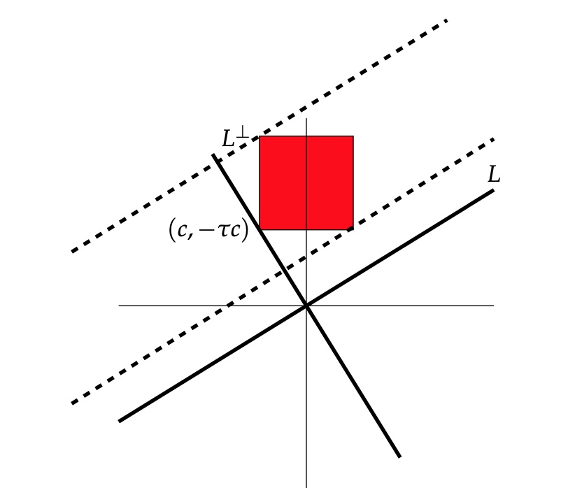
The window $W$ will be the strip, parallel with $L$ with basis $\pi^{\perp}(H_{\vec{\gamma}})$.
We cut the standard lattice $\mathbb{Z}^2$, of all points with integer coordinates in the plane, by retricting to the window $\mathcal{P}=\mathbb{Z}^2 \cap W$.
Next, we project $\mathcal{P}$ onto the line $L$, and we get a set of endpoints of intervals which divide the line $L$ into short intervals of length $\tfrac{1}{\sqrt{1+\tau^2}}$ and long intervals of length $\tfrac{\tau}{\sqrt{1+\tau^2}}$.
For $(a,b) \in W$, the interval will be short if $(a,b+1) \in W$ and long if $(a+1,b) \in W$.
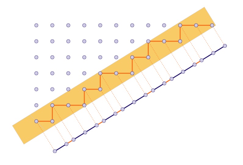
Because these intervals differ by a factor $\tau$ in length, we get a tiling of the line by short intervals $S$ and long intervals $L$. It is easy to see that they satisfy the gluing restrictions (remember, no two consecutive short intervals and no three consecutive long intervals): the horizontal width of the window $W$ is $1+\tau \approx 2.618$ (so there cannot be three consecutive long intervals in the projection) and the vertical width of the window $W$ is $1+\tfrac{1}{\tau} = \tau \approx 1.618$ so there cannot be two consecutive short intervals in the projection.
Ready for the punchline?
The sequence obtained from projecting $\mathcal{P}$ is equal to the sequence $P_{(1+\tau^2)c}$. So, we get all musical sequences of this form from the cut-and-project method!
On $L^{\perp}$ the two end-points of the window are
\[
\begin{cases}
\pi^{\perp}(c+1,-\tau c) = (\frac{(1+\tau^2)c+1}{1+\tau^2},- \tau \frac{(1+\tau^2)c+1}{1+\tau^2}) \\
\pi^{\perp}(c,-\tau c+1) = (\frac{(1+\tau^2)c-\tau}{1+\tau^2},-\tau \frac{(1+\tau^2)c-\tau}{1+\tau^2})
\end{cases} \]
Therefore, a point $(a,b) \in \mathbb{Z}^2$ lies in the window $W$ if and only if
\[
(1+\tau^2)c-\tau < a-\tau b < (1+\tau^2)c+1 \]
or equivalently, if
\[
(1+\tau^2)c+(b-1)\tau < a < (1+\tau^2)c+b \tau + 1 \]
Observe that
\[
\lceil (1+\tau^2)c + b\tau \rceil - \lceil (1+\tau^2)c+(b-1)\tau \rceil = P_{(1+\tau^2)c}(b-1) + 1 \in \{ 1,2 \} \]
We separate the two cases:
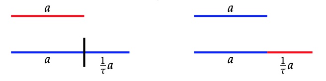
(1) : If $\lceil (1+\tau^2)c + (b+1)\tau \rceil - \lceil (1+\tau^2)c+b \tau \rceil =1$, then there must be an integer $a$ such that $(1+\tau^2)c +(b+1) \tau -1 < a < (1+\tau^2) b+1$, and this forces $\lceil (1+\tau^2)c + (b+2)\tau \rceil - \lceil (1+\tau^2)c+(b+1)\tau \rceil =2$. With $b_i = (1+\tau^2)c+(b+i)\tau$ and $d_i = b_i+1$ we have the situation

and from the inequalities above this implies that both $(a+1,b+1)$ and $(a+1,b+2)$ are in $W$, giving a short interval $S$ in the projection.
(2) : If $\lceil (1+\tau^2)c + (b+1)\tau \rceil – \lceil (1+\tau^2)c+b \tau \rceil =1$, then there must be an integer $a$ such that $(1+\tau^2)c+b \tau < a < (1+\tau^2)cv + (b+1)\tau -1$, giving the situation

giving from the inequalities that both $(a+1,b+1)$ and $(a+2,b+1)$ are in $W$, giving a long interval $L$ in the projection, finishing the proof.
Leave a Comment