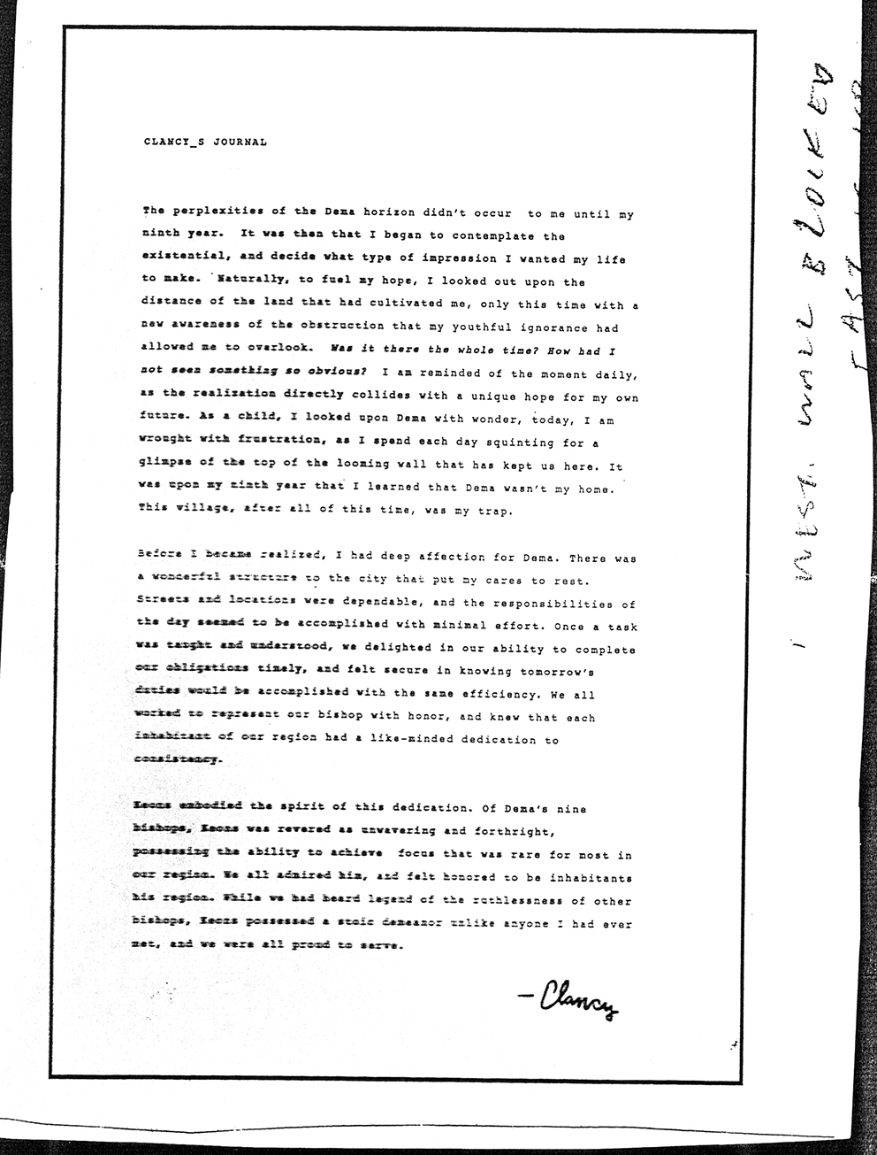
There’s this band Twenty One Pilots and they’ve woven a complicated story around some of their albums, notably Blurryface, Trench, and Scaled and Icy.
Since Trench, an important component of that story is the Bourbaki group, so I’m just curious whether the few things I know about them can help to clarify parts in the TØP- storyline.
Pretty pointless, I know, as no artistic project will follow blindly historical facts. But hey, as long as I discover new things I’ll keep going.
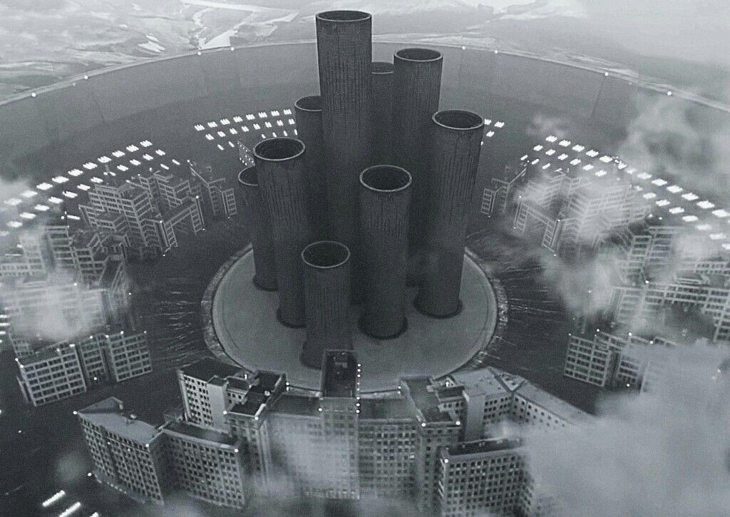
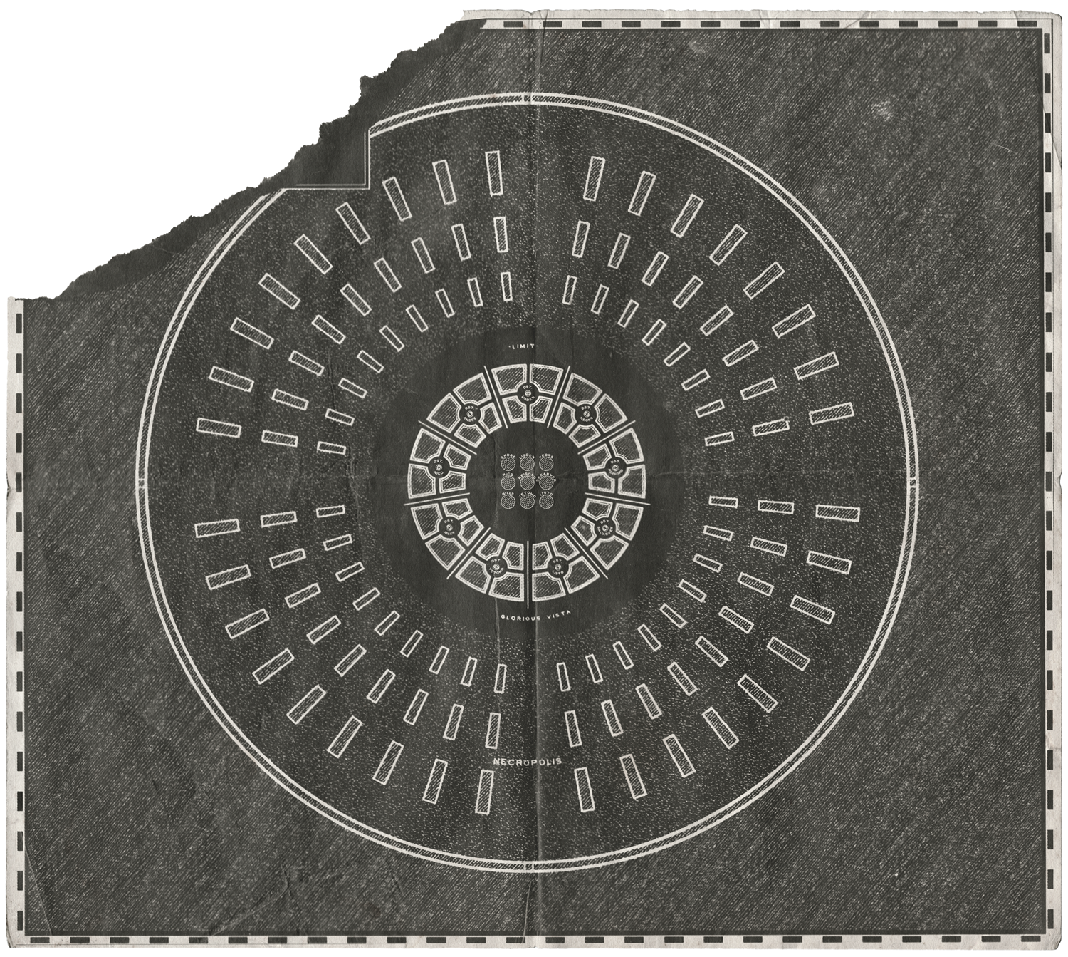
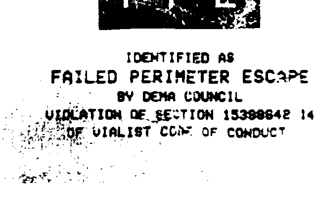
The story’s about a City of Dema, ruled by nine Bishops installing a terror regime called Vialism, and a land outside the city walls, called Trench, to which citizens would like to escape.
Think of Dema as an extremely toxic environment from which you need to escape to a safe place, let’s call it Trench.
Sadly, too often survivors from abusive settings later on create their own toxic environment, abusive to others.
So, Dema-escapees to Trench should always be wary of the danger of creating a new Dema for others.
It is very hard to break these Dema2Trench cycles of violence. That’s probably why the map of the City of Dema is circular.
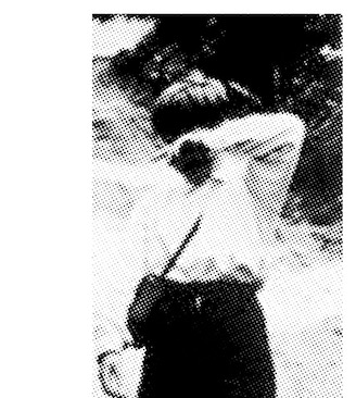
Let’s start with these two photos not (yet) in the Dema-lore:
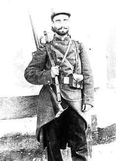
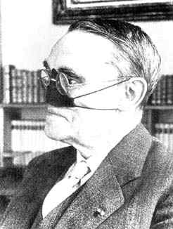
Both pictures are of the French mathematician Gaston Julia.
Julia graduated from the ENS in 1914, so was among the worst victims of the military regime Lavisse installed at the ENS. He was mobilised but hadn’t yet completed his second year of military training. That was shortened to just 5 months, after which we has send as a second lieutenant to the war.
In January 1915 he was seriously wounded in his face, had to undergo a series of operations and for the rest of his life he resigned himself to wearing a leather strap around the area where his nose had been.
He ran a weekly seminar from 1933 till 1939, the Seminaire Julia, to which the Bourbaki core members contributed a vast number of lectures.
Until 1937-38 (so just before the Dieulefit Bourbaki congress) the Bourbakis felt happy citizens of Julia’s Seminar/Dema. But then they discovered his political agenda and were expelled from it, or escaped from it depending on the version.
Jean Leray convinced Julia that it was a terrible mistake to let his seminar run by Bourbaki, and that things would go much better if he ran it. Julia expelled Bourbaki from the seminar, changed its name to ‘ Cercle mathématique de l’École normale supérieure’ and moved the venue from the IHP to the ENS. The attendants of this seminar were younger and less international that in the preceding years, hence more malleable to his political ideas.
Another reason for the break-up between Bourbaki and Julia was that they reproached him of attending in June 1937 the festivities of the bicentennial of the University of Gottingen, which were seen as pure propaganda for the Nazi-regime.
During WW2, Julia collaborated with the occupying Nazi-regime in that he tried to find French mathematicians to contribute to the Zentralblatt. After the war he was briefly suspended for this.
Much more on the Julia seminar and the break-up with Bourbaki can be read in the thesis by Gatien Ricotier ‘Projets collectifs et personnels autour de Bourbaki dans les années 1930 à 1950’, and Michele Audin’s book on the Julia Seminar.
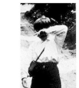
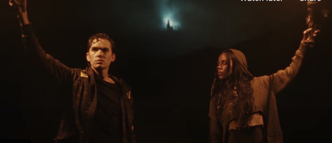
Let us compare Julia’s photographs to these two in Dema-lore:

Is it a coincidence that Clancy in Trench has a scar on his nose? Is it a coincidence that the black paint on some of the Bishop’s faces looks a lot like Julia’s mask?
Can it be that victims of one Dema-era become Bishops in a next era?
This repetitiveness of Dema-environments also indicates the importance of Bishop Andre. Recall that all the Bishops’ names (except for Nico) come from concatenations of word-parts in the lyrics of the songs on the Blurryface album.
ANDRE comes from ‘..AND REpeat’ in Fairly local:
Tomorrow I’ll keep a beat
And repeat yesterday’s dance
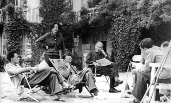
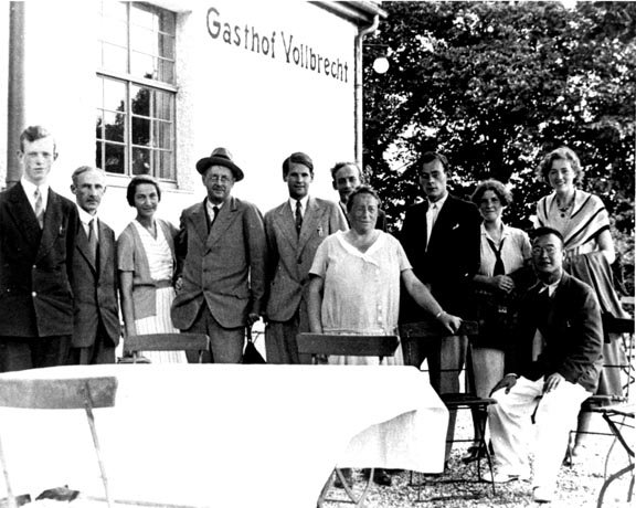
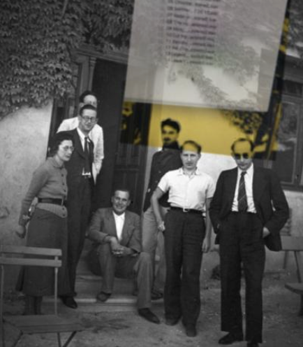
In view of this, let’s have another look at the two Bourbaki-related photographs that appeared in the run up to the Trench-album:


On the left is the photo of the Dieulefit/Beauvallon 1938 meeting, which is on the Bourbaki Wikipedia page, and was on the desktop of Tyler Joseph.
On the right a photo of Andre Weil together with a girl, according to Wikipedia the picture dates from 1956. I’m pretty certain it was taken in the summer of 1957, and that the girl is Mireille Cartan, the second youngest daughter of Henri Cartan. Not that any of this matters, TØP-wise. A clipping of the girl was among the material originally posted at the dmaorg.info site.
In 1938, Andre Weil was a victim of Lavisse’s Dema. His year was the last one getting a military training to become reserve officers in the French infantry/artillery (as were Cartan, Dieudonne and Delsarte).
When France would mobilise they were forced to return to Dema (military service) and lead their bataljons as second lieutenants into war. All of them, except for Weil, did this.
Weil escaped to Trench (Finland), and was taken back to Dema, and imprisonment.
In 1957, Bourbaki dominated much of French mathematical life, and certainly its influence in Paris was suffocating for aspiring math-students. A good read on this is Jacques Roubaud’s Mathematique.
Bourbaki has turned French mathematics (and beyond) into its own Dema, and Andre Weil certainly was one of the more important Bishops of it.
In this series:
- Bourbaki and TØP : East is up
- Bourbaki = Bishops or Banditos?
- Where’s Bourbaki’s Dema?
- Weil photos used in Dema-lore
- Dema2Trench, AND REpeat
- TØP PhotoShop mysteries
- 9 Bourbaki founding members, really?
- Bourbaki and Dema, two remarks
- Clancy and Nancago
- What about Simone Weil?
- Vialism versus Weilism
- The dangerous bend symbol


+(Large).JPG)

.jpg)