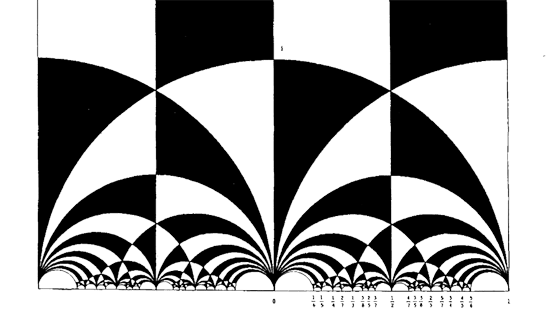
 The black&white psychedelic picture on the left of a tessellation of the hyperbolic upper-halfplane, was called the Dedekind tessellation in this post, following the reference given by John Stillwell in his excellent paper Modular Miracles, The American Mathematical Monthly, 108 (2001) 70-76.
But is this correct terminology? Nobody else uses it apparently. So, let’s try to track down the earliest depiction of this tessellation in the literature…
 Stillwell refers to Richard Dedekind‘s 1877 paper “Schreiben an Herrn Borchard uber die Theorie der elliptische Modulfunktionen”, which appeared beginning of september 1877 in Crelle’s journal (Journal fur die reine und angewandte Mathematik, Bd. 83, 265-292).
There are a few odd things about this paper. To start, it really is the transcript of a (lengthy) letter to Herrn Borchardt (at first, I misread the recipient as Herrn Borcherds which would be really weird…), written on June 12th 1877, just 2 and a half months before it appeared… Even today in the age of camera-ready-copy it would probably take longer.
There isn’t a single figure in the paper, but, it is almost impossible to follow Dedekind’s arguments without having a mental image of the tessellation. He gives a fundamental domain for the action of the modular group $\Gamma = PSL_2(\mathbb{Z}) $ on the hyperbolic upper-half plane (a fact already known to Gauss) and goes on in section 3 to give a one-to-one mapping between this domain and the complex plane using what he calls the ‘valenz’ function $v $ (which is our modular function $j $, making an appearance in moonshine, and responsible for the black&white tessellation, the two colours corresponding to pre-images of the upper or lower half-planes).
Then there is this remarkable opening sentence.
Sie haben mich aufgefordert, eine etwas ausfuhrlichere Darstellung der Untersuchungen auszuarbeiten, von welchen ich, durch das Erscheinen der Abhandlung von Fuchs veranlasst, mir neulich erlaubt habe Ihnen eine kurze Ubersicht mitzuteilen; indem ich Ihrer Einladung hiermit Folge leiste, beschranke ich mich im wesentlichen auf den Teil dieser Untersuchungen, welcher mit der eben genannten Abhandlung zusammenhangt, und ich bitte Sie auch, die Ubergehung einiger Nebenpunkte entschuldigen zu wollen, da es mir im Augenblick an Zeit fehlt, alle Einzelheiten auszufuhren.
Well, just try to get a paper (let alone a letter) accepted by Crelle’s Journal with an opening line like : “I’ll restrict to just a few of the things I know, and even then, I cannot be bothered to fill in details as I don’t have the time to do so right now!” But somehow, Dedekind got away with it.
So, who was this guy Borchardt? How could this paper be published so swiftly? And, what might explain this extreme ‘je m’en fous’-opening ?
 Carl Borchardt was a Berlin mathematician whose main claim to fame seems to be that he succeeded Crelle in 1856 as main editor of the ‘Journal fur reine und…’ until 1880 (so in 1877 he was still in charge, explaining the swift publication). It seems that during this time the ‘Journal’ was often referred to as “Borchardt’s Journal” or in France as “Journal de M Borchardt”. After Borchardt’s death, the Journal für die Reine und Angewandte Mathematik again became known as Crelle’s Journal.
As to the opening sentence, I have a toy-theory of what was going on. In 1877 a bitter dispute was raging between Kronecker (an editor for the Journal and an important one as he was the one succeeding Borchardt when he died in 1880) and Cantor. Cantor had published most of his papers at Crelle and submitted his latest find : there is a one-to-one correspondence between points in the unit interval [0,1] and points of d-dimensional space! Kronecker did everything in his power to stop that paper to the extend that Cantor wanted to retract it and submit it elsewhere. Dedekind supported Cantor and convinced him not to retract the paper and used his influence to have the paper published in Crelle in 1878. Cantor greatly resented Kronecker’s opposition to his work and never submitted any further papers to Crelle’s Journal.
Clearly, Borchardt was involved in the dispute and it is plausible that he ‘invited’ Dedekind to submit a paper on his old results in the process. As a further peace offering, Dedekind included a few ‘nice’ words for Kronecker
Bei meiner Versuchen, tiefer in diese mir unentbehrliche Theorie einzudringen und mir einen einfachen Weg zu den ausgezeichnet schonen Resultaten von Kronecker zu bahnen, die leider noch immer so schwer zuganglich sind, enkannte ich sogleich…
Probably, Dedekind was referring to Kronecker’s relation between class groups of quadratic imaginary fields and the j-function, see the miracle of 163. As an added bonus, Dedekind was elected to the Berlin academy in 1880…
Anyhow, no visible sign of ‘Dedekind’s’ tessellation in the 1877 Dedekind paper, so, we have to look further. I’m fairly certain to have found the earliest depiction of the black&white tessellation (if you have better info, please drop a line). Here it is
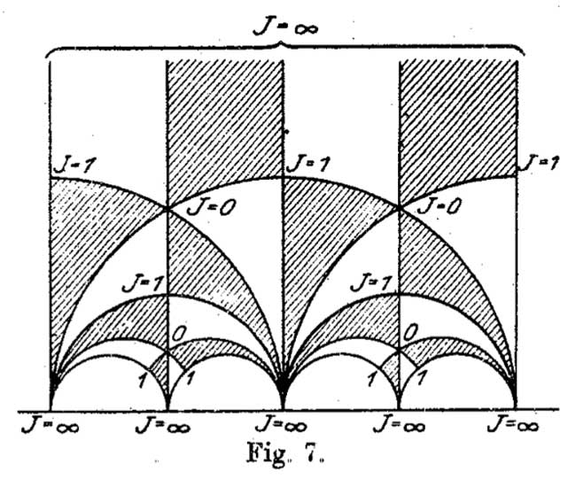
It is figure 7 in Felix Klein‘s paper “Uber die Transformation der elliptischen Funktionen und die Auflosung der Gleichungen funften Grades” which appeared in may 1878 in the Mathematische Annalen (Bd. 14 1878/79). He even adds the j-values which make it clear why black triangles should be oriented counter-clockwise and white triangles clockwise. If Klein would still be around today, I’m certain he’d be a metapost-guru.
So, perhaps the tessellation should be called Klein’s tessellation??
Well, not quite. Here’s what Klein writes wrt. figure 7
Diese Figur nun – welche die eigentliche Grundlage fur das Nachfolgende abgibt – ist eben diejenige, von der Dedekind bei seiner Darstellung ausgeht. Er kommt zu ihr durch rein arithmetische Betrachtung.
Case closed : Klein clearly acknowledges that Dedekind did have this picture in mind when writing his 1877 paper!
But then, there are a few odd things about Klein’s paper too, and, I do have a toy-theory about this as well… (tbc)
3 Comments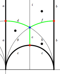
 Another combinatorial gadget assigned to the fundamental domain is the
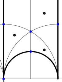
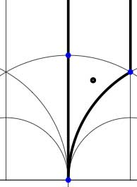
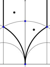
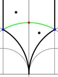
 In these cases the fundamental domain consists of 6 triangles with the indicated vertices (the blue dots). The distinction between the two is that in the first case, one identifies the two edges of the left, resp. bottom, resp. right boundary (so, in particular, 0,1 and $\infty $ are identified) whereas in the second one identifies the two edges of the left boundary and identifies the edges of the bottom with those of the right boundary (here, 0 is identified only with $\infty $ but also $1+i $ is indetified with $\frac{1}{2}+\frac{1}{2}i $).
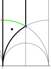
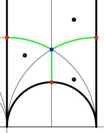 In both cases the dessin seems to be the same (and given by the picture on the right). However, in the first case all three red vertices are distinct hence there are no internal red vertices in this case whereas in the second case we should identify the bottom and right-hand red vertex which then becomes an internal red vertex of the dessin!