The Monster is the largest of the 26 sporadic simple groups and has order
808 017 424 794 512 875 886 459 904 961 710 757 005 754 368 000 000 000
= 2^46 3^20 5^9 7^6 11^2 13^3 17 19 23 29 31 41 47 59 71.
It is not so much the size of its order that makes it hard to do actual calculations in the monster, but rather the dimensions of its smallest non-trivial irreducible representations (196 883 for the smallest, 21 296 876 for the next one, and so on).
In characteristic two there is an irreducible representation of one dimension less (196 882) which appears to be of great use to obtain information. For example, Robert Wilson used it to prove that The Monster is a Hurwitz group. This means that the Monster is generated by two elements g and h satisfying the relations
$g^2 = h^3 = (gh)^7 = 1 $
Geometrically, this implies that the Monster is the automorphism group of a Riemann surface of genus g satisfying the Hurwitz bound 84(g-1)=#Monster. That is,
g=9619255057077534236743570297163223297687552000000001=42151199 * 293998543 * 776222682603828537142813968452830193
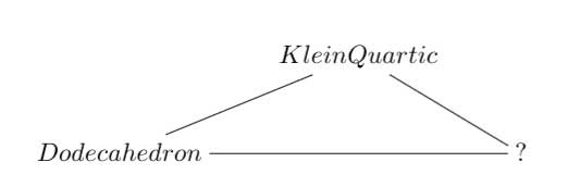
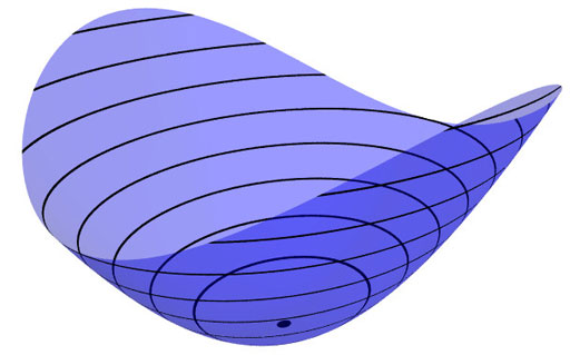
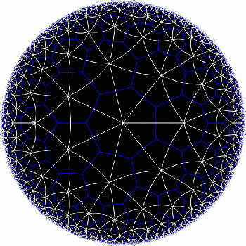
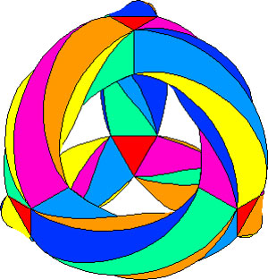
Or, in analogy with the Klein quartic which can be constructed from 24 heptagons in the tiling of the hyperbolic plane, there is a finite region of the hyperbolic plane, tiled with heptagons, from which we can construct this monster curve by gluing the boundary is a specific way so that we get a Riemann surface with exactly 9619255057077534236743570297163223297687552000000001 holes. This finite part of the hyperbolic tiling (consisting of #Monster/7 heptagons) we’ll call the empire of the monster and we’d love to describe it in more detail.
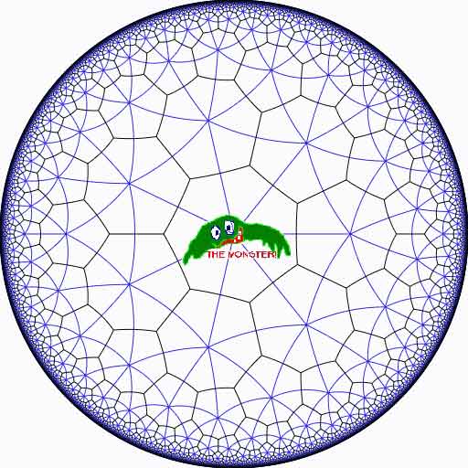
Look at the half-edges of all the heptagons in the empire (the picture above learns that every edge in cut in two by a blue geodesic). They are exactly #Monster such half-edges and they form a dessin d’enfant for the monster-curve.
If we label these half-edges by the elements of the Monster, then multiplication by g in the monster interchanges the two half-edges making up a heptagonal edge in the empire and multiplication by h in the monster takes a half-edge to the one encountered first by going counter-clockwise in the vertex of the heptagonal tiling. Because g and h generated the Monster, the dessin of the empire is just a concrete realization of the monster.
Because g is of order two and h is of order three, the two permutations they determine on the dessin, gives a group epimorphism $C_2 \ast C_3 = PSL_2(\mathbb{Z}) \rightarrow \mathbb{M} $ from the modular group $PSL_2(\mathbb{Z}) $ onto the Monster-group.
In noncommutative geometry, the group-algebra of the modular group $\mathbb{C} PSL_2 $ can be interpreted as the coordinate ring of a noncommutative manifold (because it is formally smooth in the sense of Kontsevich-Rosenberg or Cuntz-Quillen) and the group-algebra of the Monster $\mathbb{C} \mathbb{M} $ itself corresponds in this picture to a finite collection of ‘points’ on the manifold. Using this geometric viewpoint we can now ask the question What does the Monster see of the modular group?
To make sense of this question, let us first consider the commutative equivalent : what does a point P see of a commutative variety X?
Evaluation of polynomial functions in P gives us an algebra epimorphism $\mathbb{C}[X] \rightarrow \mathbb{C} $ from the coordinate ring of the variety $\mathbb{C}[X] $ onto $\mathbb{C} $ and the kernel of this map is the maximal ideal $\mathfrak{m}_P $ of
$\mathbb{C}[X] $ consisting of all functions vanishing in P.
Equivalently, we can view the point $P= \mathbf{spec}~\mathbb{C}[X]/\mathfrak{m}_P $ as the scheme corresponding to the quotient $\mathbb{C}[X]/\mathfrak{m}_P $. Call this the 0-th formal neighborhood of the point P.
This sounds pretty useless, but let us now consider higher-order formal neighborhoods. Call the affine scheme $\mathbf{spec}~\mathbb{C}[X]/\mathfrak{m}_P^{n+1} $ the n-th forml neighborhood of P, then the first neighborhood, that is with coordinate ring $\mathbb{C}[X]/\mathfrak{m}_P^2 $ gives us tangent-information. Alternatively, it gives the best linear approximation of functions near P.
The second neighborhood $\mathbb{C}[X]/\mathfrak{m}_P^3 $ gives us the best quadratic approximation of function near P, etc. etc.
These successive quotients by powers of the maximal ideal $\mathfrak{m}_P $ form a system of algebra epimorphisms
$\ldots \frac{\mathbb{C}[X]}{\mathfrak{m}_P^{n+1}} \rightarrow \frac{\mathbb{C}[X]}{\mathfrak{m}_P^{n}} \rightarrow \ldots \ldots \rightarrow \frac{\mathbb{C}[X]}{\mathfrak{m}_P^{2}} \rightarrow \frac{\mathbb{C}[X]}{\mathfrak{m}_P} = \mathbb{C} $
and its inverse limit $\underset{\leftarrow}{lim}~\frac{\mathbb{C}[X]}{\mathfrak{m}_P^{n}} = \hat{\mathcal{O}}_{X,P} $ is the completion of the local ring in P and contains all the infinitesimal information (to any order) of the variety X in a neighborhood of P. That is, this completion $\hat{\mathcal{O}}_{X,P} $ contains all information that P can see of the variety X.
In case P is a smooth point of X, then X is a manifold in a neighborhood of P and then this completion
$\hat{\mathcal{O}}_{X,P} $ is isomorphic to the algebra of formal power series $\mathbb{C}[[ x_1,x_2,\ldots,x_d ]] $ where the $x_i $ form a local system of coordinates for the manifold X near P.
Right, after this lengthy recollection, back to our question what does the monster see of the modular group? Well, we have an algebra epimorphism
$\pi~:~\mathbb{C} PSL_2(\mathbb{Z}) \rightarrow \mathbb{C} \mathbb{M} $
and in analogy with the commutative case, all information the Monster can gain from the modular group is contained in the $\mathfrak{m} $-adic completion
$\widehat{\mathbb{C} PSL_2(\mathbb{Z})}_{\mathfrak{m}} = \underset{\leftarrow}{lim}~\frac{\mathbb{C} PSL_2(\mathbb{Z})}{\mathfrak{m}^n} $
where $\mathfrak{m} $ is the kernel of the epimorphism $\pi $ sending the two free generators of the modular group $PSL_2(\mathbb{Z}) = C_2 \ast C_3 $ to the permutations g and h determined by the dessin of the pentagonal tiling of the Monster’s empire.
As it is a hopeless task to determine the Monster-empire explicitly, it seems even more hopeless to determine the kernel $\mathfrak{m} $ let alone the completed algebra… But, (surprise) we can compute $\widehat{\mathbb{C} PSL_2(\mathbb{Z})}_{\mathfrak{m}} $ as explicitly as in the commutative case we have $\hat{\mathcal{O}}_{X,P} \simeq \mathbb{C}[[ x_1,x_2,\ldots,x_d ]] $ for a point P on a manifold X.
Here the details : the quotient $\mathfrak{m}/\mathfrak{m}^2 $ has a natural structure of $\mathbb{C} \mathbb{M} $-bimodule. The group-algebra of the monster is a semi-simple algebra, that is, a direct sum of full matrix-algebras of sizes corresponding to the dimensions of the irreducible monster-representations. That is,
$\mathbb{C} \mathbb{M} \simeq \mathbb{C} \oplus M_{196883}(\mathbb{C}) \oplus M_{21296876}(\mathbb{C}) \oplus \ldots \ldots \oplus M_{258823477531055064045234375}(\mathbb{C}) $
with exactly 194 components (the number of irreducible Monster-representations). For any $\mathbb{C} \mathbb{M} $-bimodule $M $ one can form the tensor-algebra
$T_{\mathbb{C} \mathbb{M}}(M) = \mathbb{C} \mathbb{M} \oplus M \oplus (M \otimes_{\mathbb{C} \mathbb{M}} M) \oplus (M \otimes_{\mathbb{C} \mathbb{M}} M \otimes_{\mathbb{C} \mathbb{M}} M) \oplus \ldots \ldots $


and applying the formal neighborhood theorem for formally smooth algebras (such as $\mathbb{C} PSL_2(\mathbb{Z}) $) due to Joachim Cuntz (left) and Daniel Quillen (right) we have an isomorphism of algebras
$\widehat{\mathbb{C} PSL_2(\mathbb{Z})}_{\mathfrak{m}} \simeq \widehat{T_{\mathbb{C} \mathbb{M}}(\mathfrak{m}/\mathfrak{m}^2)} $
where the right-hand side is the completion of the tensor-algebra (at the unique graded maximal ideal) of the $\mathbb{C} \mathbb{M} $-bimodule $\mathfrak{m}/\mathfrak{m}^2 $, so we’d better describe this bimodule explicitly.
Okay, so what’s a bimodule over a semisimple algebra of the form $S=M_{n_1}(\mathbb{C}) \oplus \ldots \oplus M_{n_k}(\mathbb{C}) $? Well, a simple S-bimodule must be either (1) a factor $M_{n_i}(\mathbb{C}) $ with all other factors acting trivially or (2) the full space of rectangular matrices $M_{n_i \times n_j}(\mathbb{C}) $ with the factor $M_{n_i}(\mathbb{C}) $ acting on the left, $M_{n_j}(\mathbb{C}) $ acting on the right and all other factors acting trivially.
That is, any S-bimodule can be represented by a quiver (that is a directed graph) on k vertices (the number of matrix components) with a loop in vertex i corresponding to each simple factor of type (1) and a directed arrow from i to j corresponding to every simple factor of type (2).
That is, for the Monster, the bimodule $\mathfrak{m}/\mathfrak{m}^2 $ is represented by a quiver on 194 vertices and now we only have to determine how many loops and arrows there are at or between vertices.
Using Morita equivalences and standard representation theory of quivers it isn’t exactly rocket science to determine that the number of arrows between the vertices corresponding to the irreducible Monster-representations $S_i $ and $S_j $ is equal to
$dim_{\mathbb{C}}~Ext^1_{\mathbb{C} PSL_2(\mathbb{Z})}(S_i,S_j)-\delta_{ij} $
Now, I’ve been wasting a lot of time already here explaining what representations of the modular group have to do with quivers (see for example here or some other posts in the same series) and for quiver-representations we all know how to compute Ext-dimensions in terms of the Euler-form applied to the dimension vectors.
Right, so for every Monster-irreducible $S_i $ we have to determine the corresponding dimension-vector $~(a_1,a_2;b_1,b_2,b_3) $ for the quiver
$\xymatrix{ & & & &
\vtx{b_1} \\ \vtx{a_1} \ar[rrrru]^(.3){B_{11}} \ar[rrrrd]^(.3){B_{21}}
\ar[rrrrddd]_(.2){B_{31}} & & & & \\ & & & & \vtx{b_2} \\ \vtx{a_2}
\ar[rrrruuu]_(.7){B_{12}} \ar[rrrru]_(.7){B_{22}}
\ar[rrrrd]_(.7){B_{23}} & & & & \\ & & & & \vtx{b_3}} $
Now the dimensions $a_i $ are the dimensions of the +/-1 eigenspaces for the order 2 element g in the representation and the $b_i $ are the dimensions of the eigenspaces for the order 3 element h. So, we have to determine to which conjugacy classes g and h belong, and from Wilson’s paper mentioned above these are classes 2B and 3B in standard Atlas notation.
So, for each of the 194 irreducible Monster-representations we look up the character values at 2B and 3B (see below for the first batch of those) and these together with the dimensions determine the dimension vector $~(a_1,a_2;b_1,b_2,b_3) $.
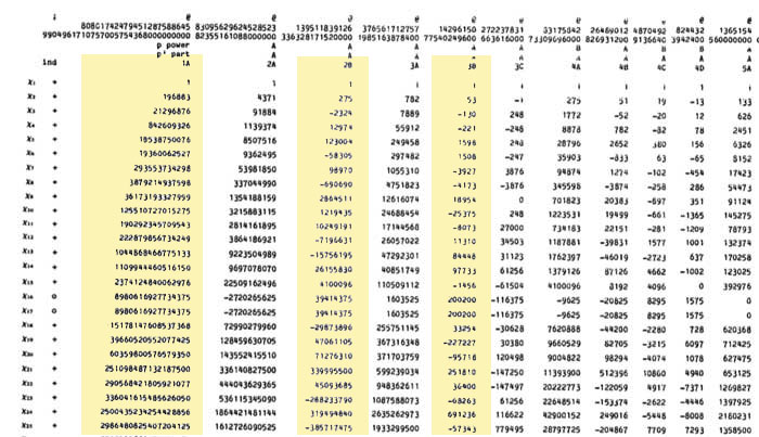
For example take the 196883-dimensional irreducible. Its 2B-character is 275 and the 3B-character is 53. So we are looking for a dimension vector such that $a_1+a_2=196883, a_1-275=a_2 $ and $b_1+b_2+b_3=196883, b_1-53=b_2=b_3 $ giving us for that representation the dimension vector of the quiver above $~(98579,98304,65663,65610,65610) $.
Okay, so for each of the 194 irreducibles $S_i $ we have determined a dimension vector $~(a_1(i),a_2(i);b_1(i),b_2(i),b_3(i)) $, then standard quiver-representation theory asserts that the number of loops in the vertex corresponding to $S_i $ is equal to
$dim(S_i)^2 + 1 – a_1(i)^2-a_2(i)^2-b_1(i)^2-b_2(i)^2-b_3(i)^2 $
and that the number of arrows from vertex $S_i $ to vertex $S_j $ is equal to
$dim(S_i)dim(S_j) – a_1(i)a_1(j)-a_2(i)a_2(j)-b_1(i)b_1(j)-b_2(i)b_2(j)-b_3(i)b_3(j) $
This data then determines completely the $\mathbb{C} \mathbb{M} $-bimodule $\mathfrak{m}/\mathfrak{m}^2 $ and hence the structure of the completion $\widehat{\mathbb{C} PSL_2}_{\mathfrak{m}} $ containing all information the Monster can gain from the modular group.
But then, one doesn’t have to go for the full regular representation of the Monster. Any faithful permutation representation will do, so we might as well go for the one of minimal dimension.
That one is known to correspond to the largest maximal subgroup of the Monster which is known to be a two-fold extension $2.\mathbb{B} $ of the Baby-Monster. The corresponding permutation representation is of dimension 97239461142009186000 and decomposes into Monster-irreducibles
$S_1 \oplus S_2 \oplus S_4 \oplus S_5 \oplus S_9 \oplus S_{14} \oplus S_{21} \oplus S_{34} \oplus S_{35} $
(in standard Atlas-ordering) and hence repeating the arguments above we get a quiver on just 9 vertices! The actual numbers of loops and arrows (I forgot to mention this, but the quivers obtained are actually symmetric) obtained were found after laborious computations mentioned in this post and the details I’ll make avalable here.
Anyone who can spot a relation between the numbers obtained and any other part of mathematics will obtain quantities of genuine (ie. non-Inbev) Belgian beer…
8 Comments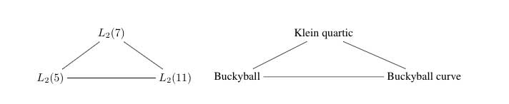

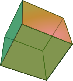
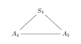
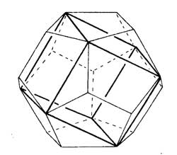
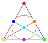 Shifting perspective, we can repeat this for each of the seven different colors. That is, we have seven truncated cubes in the Klein quartic. On each of them a copy of $S_4 $ acts and these subgroups form one of the two conjugacy classes of $S_4 $ in the group $L_2(7) $. The colors of the triangles of these seven truncated cubes are indicated by bullets in the picture above on the right. The other conjugacy class of $S_4 $’s act on ‘truncated anti-cubes’ which also come in seven bunches of which the color is indicated by a square in that picture.
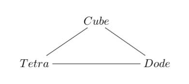
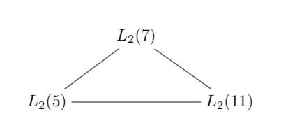
 Referring to the triple of exceptional Galois groups $L_2(5),L_2(7),L_2(11) $ and its connection to the Platonic solids I