By now, everyone remotely interested in Connes’ approach to the Riemann hypothesis, knows the _one line mantra_
one can use noncommutative geometry to extend Weil’s proof of the Riemann-hypothesis in the function field case to that of number fields
But, can one go beyond this sound-bite in a series of blog posts? A few days ago, I was rather optimistic, but now, after reading-up on the Connes-Consani-Marcolli project, I feel overwhelmed by the sheer volume of their work (and by my own ignorance of key tools in the approach). The most recent account takes up half of the 700+ pages of the book Noncommutative Geometry, Quantum Fields and Motives by Alain Connes and Matilde Marcolli…
So let us set a more modest goal and try to understand one of the first papers Alain Connes wrote about the RH : Noncommutative geometry and the Riemann zeta function. It is only 24 pages long and relatively readable. But even then, the reader needs to know about class field theory, the classification of AF-algebras, Hecke algebras, etc. etc. Most of these theories take a book to explain. For example, the first result he mentions is the main result of local class field theory which appears only towards the end of the 200+ pages of Jean-Pierre Serre’s Local Fields, itself a somewhat harder read than the average blogpost…
Anyway, we will see how far we can get. Here’s the plan : I’ll take the heart-bit of their approach : the Bost-Connes system, and will try to understand it from an algebraist’s viewpoint. Today we will introduce the groups involved and describe their cosets.
For any commutative ring $R $ let us consider the group of triangular $2 \times 2 $ matrices of the form
$P_R = { \begin{bmatrix} 1 & b \\ 0 & a \end{bmatrix}~|~b \in R, a \in R^* } $
(that is, $a $ in an invertible element in the ring $R $). This is really an affine group scheme defined over the integers, that is, the coordinate ring
$\mathbb{Z}[P] = \mathbb{Z}[x,x^{-1},y] $ becomes a Hopf algebra with comultiplication encoding the group-multiplication. Because
$\begin{bmatrix} 1 & b_1 \\ 0 & a_1 \end{bmatrix} \begin{bmatrix} 1 & b_2 \\ 0 & a_2 \end{bmatrix} = \begin{bmatrix} 1 & 1 \times b_2 + b_1 \times a_2 \\ 0 & a_1 \times a_2 \end{bmatrix} $
we have $\Delta(x) = x \otimes x $ and $\Delta(y) = 1 \otimes y + y \otimes x $, or $x $ is a group-like element whereas $y $ is a skew-primitive. If $R \subset \mathbb{R} $ is a subring of the real numbers, we denote by $P_R^+ $ the subgroup of $P_R $ consisting of all matrices with $a > 0 $. For example,
$\Gamma_0 = P_{\mathbb{Z}}^+ = { \begin{bmatrix} 1 & n \\ 0 & 1 \end{bmatrix}~|~n \in \mathbb{Z} } $
which is a subgroup of $\Gamma = P_{\mathbb{Q}}^+ $ and our first job is to describe the cosets.
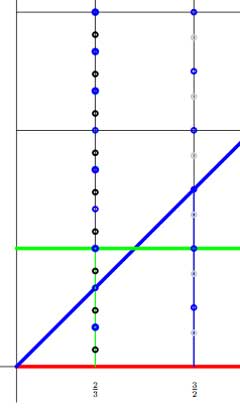 The left cosets $\Gamma / \Gamma_0 $ are the subsets $\gamma \Gamma_0 $ with $\gamma \in \Gamma $. But,
$\begin{bmatrix} 1 & b \\ 0 & a \end{bmatrix} \begin{bmatrix} 1 & n \\ 0 & 1 \end{bmatrix} = \begin{bmatrix} 1 & b+n \\ 0 & a \end{bmatrix} $
so if we represent the matrix $\gamma = \begin{bmatrix} 1 & b \\ 0 & a \end{bmatrix} $ by the point $~(a,b) $ in the right halfplane, then for a given positive rational number $a $ the different cosets are represented by all $b \in [0,1) \cap \mathbb{Q} = \mathbb{Q}/\mathbb{Z} $. Hence, the left cosets are all the rational points in the region between the red and green horizontal lines. For fixed $a $ the cosets correspond to the rational points in the green interval (such as over $\frac{2}{3} $ in the picture on the left.
Similarly, the right cosets $\Gamma_0 \backslash \Gamma $ are the subsets $\Gamma_0 \gamma $ and as
$\begin{bmatrix} 1 & n \\ 0 & 1 \end{bmatrix} \begin{bmatrix} 1 & b \\ 0 & a \end{bmatrix} = \begin{bmatrix} 1 & b+na \\ 0 & a \end{bmatrix} $
we see similarly that the different cosets are precisely the rational points in the region between the lower red horizontal and the blue diagonal line. So, for fixed $a $ they correspond to rational points in the blue interval (such as over $\frac{3}{2} $) $[0,a) \cap \mathbb{Q} $. But now, let us look at the double coset space $\Gamma_0 \backslash \Gamma / \Gamma_0 $. That is, we want to study the orbits of the action of $\Gamma_0 $, acting on the right, on the left-cosets $\Gamma / \Gamma_0 $, or equivalently, of the action of $\Gamma_0 $ acting on the left on the right-cosets $\Gamma_0 \backslash \Gamma $. The crucial observation to make is that these actions have finite orbits, or equivalently, that $\Gamma_0 $ is an almost normal subgroup of $\Gamma $ meaning that $\Gamma_0 \cap \gamma \Gamma_0 \gamma^{-1} $ has finite index in $\Gamma_0 $ for all $\gamma \in \Gamma $. This follows from
$\begin{bmatrix} 1 & n \\ 0 & 1 \end{bmatrix} \begin{bmatrix} 1 & b \\ 0 & a \end{bmatrix} \begin{bmatrix} 1 & m \\ 0 & 1 \end{bmatrix} = \begin{bmatrix} 1 & b+m+an \\ 0 & a \end{bmatrix} $
and if $n $ varies then $an $ takes only finitely many values modulo $\mathbb{Z} $ and their number depends only on the denominator of $a $. In the picture above, the blue dots lying on the line over $\frac{2}{3} $ represent the double coset
$\Gamma_0 \begin{bmatrix} 1 & \frac{2}{3} \\ 0 & \frac{2}{3} \end{bmatrix} $ and we see that these dots split the left-cosets with fixed value $a=\frac{2}{3} $ (that is, the green line-segment) into three chunks (3 being the denominator of a) and split the right-cosets (the line-segment under the blue diagonal) into two subsegments (2 being the numerator of a). Similarly, the blue dots on the line over $\frac{3}{2} $ divide the left-cosets in two parts and the right cosets into three parts.
This shows that the $\Gamma_0 $-orbits of the right action on the left cosets $\Gamma/\Gamma_0 $ for each matrix $\gamma \in \Gamma $ with $a=\frac{2}{3} $ consist of exactly three points, and we denote this by writing $L(\gamma) = 3 $. Similarly, all $\Gamma_0 $-orbits of the left action on the right cosets $\Gamma_0 \backslash \Gamma $ with this value of a consist of two points, and we write this as $R(\gamma) = 2 $.
For example, on the above picture, the black dots on the line over $\frac{2}{3} $ give the matrices in the double coset of the matrix
$\gamma = \begin{bmatrix} 1 & \frac{1}{7} \\ 0 & \frac{2}{3} \end{bmatrix} $
and the gray dots on the line over $\frac{3}{2} $ determine the elements of the double coset of
$\gamma^{-1} = \begin{bmatrix} 1 & -\frac{3}{14} \\ 0 & \frac{3}{2} \end{bmatrix} $
and one notices (in general) that $L(\gamma) = R(\gamma^{-1}) $. But then, the double cosets with $a=\frac{2}{3} $ are represented by the rational b’s in the interval $[0,\frac{1}{3}) $ and those with $a=\frac{3}{2} $ by the rational b’s in the interval $\frac{1}{2} $. In general, the double cosets of matrices with fixed $a = \frac{r}{s} $ with $~(r,s)=1 $ are the rational points in the line-segment over $a $ with $b \in [0,\frac{1}{s}) $.
That is, the Bost-Connes double coset space $\Gamma_0 \backslash \Gamma / \Gamma_0 $ are the rational points in a horrible fractal comb. Below we have drawn only the part of the dyadic values, that is when $a = \frac{r}{2^t} $ in the unit inverval
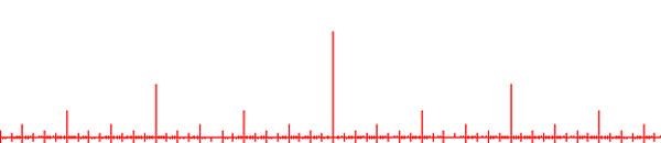
and of course we have to super-impose on it similar pictures for rationals with other powers as their denominators. Fortunately, NCG excels in describing such fractal beasts…
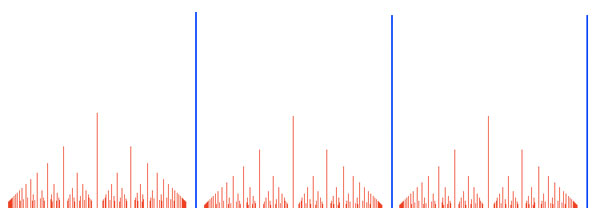
UPDATE : here is a slightly beter picture of the coset space, drawing the part over all rational numbers contained in the 15-th Farey sequence. The blue segments of length one are at 1,2,3,…
Comments