Skip to content →

Tag: the

the strange island of two truths

Last time we had a brief encounter with the island of two truths, invented by Karin Cvetko-Vah. See her posts:

On this island, false statements have truth-value $0$ (as usual), but non-false statements are not necessarily true, but can be given either truth-value $Q$ (statements which the Queen on the island prefers) or $K$ (preferred by the King).

Think of the island as Trump’s paradise where nobody is ever able to say: “Look, alternative truths are not truths. They’re falsehoods.”


Even the presence of just one ‘alternative truth’ has dramatic consequences on the rationality of your reasoning. If we know the truth-values of specific sentences, we can determine the truth-value of more complex sentences in which we use logical connectives such as $\vee$ (or), $\wedge$ (and), $\neg$ (not), and $\implies$ (then) via these truth tables:

\[
\begin{array}{c|ccc}
\downarrow~\bf{\wedge}~\rightarrow & 0 & Q & K \\
\hline
0 & 0 & 0 & 0 \\
Q & 0 & Q & Q \\
K & 0 & K & K
\end{array} \quad
\begin{array}{c|ccc}
\downarrow~\vee~\rightarrow & 0 & Q & K \\
\hline
0 & 0 & Q & K \\
Q & Q & Q & K \\
K & K & Q & K
\end{array} \]
\[
\begin{array}{c|ccc}
\downarrow~\implies~\rightarrow & 0 & Q & K \\
\hline
0 & Q & Q & K \\
Q & 0 & Q & K \\
K & 0 & Q & K
\end{array} \quad
\begin{array}{c|c}
\downarrow & \neg~\downarrow \\
\hline
0 & Q \\
Q & 0 \\
K & 0
\end{array}
\]

Note that the truth-values $Q$ and $K$ are not completely on equal footing as we have to make a choice which one of them will stand for $\neg 0$.

Common tautologies are no longer valid on this island. The best we can have are $Q$-tautologies (giving value $Q$ whatever the values of the components) or $K$-tautologies.

Here’s one $Q$-tautology (check!) : $(\neg p) \vee (\neg \neg p)$. Verify that $p \vee (\neg p)$ is neither a $Q$- nor a $K$-tautology.

Can you find any $K$-tautology at all?

Already this makes it incredibly difficult to adapt Smullyan-like Knights and Knaves puzzles to this skewed island. Last time I gave one easy example.


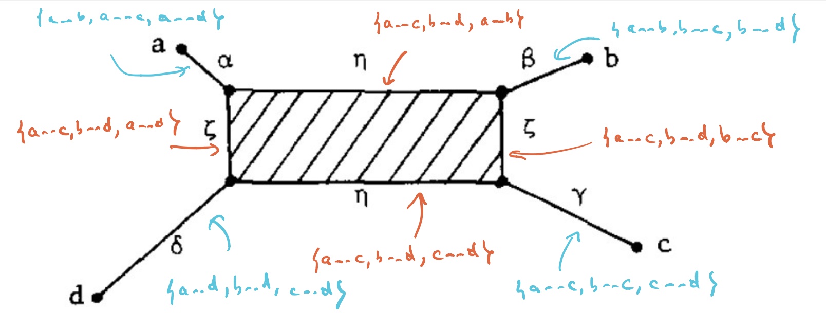
Puzzle : On an island of two truths all inhabitants are either Knaves (saying only false statements), Q-Knights (saying only $Q$-valued statements) or K-Knights (who only say $K$-valued statements).

The King came across three inhabitants, whom we will call $A$, $B$ and $C$. He asked $A$: “Are you one of my Knights?” $A$ answered, but so indistinctly that the King could not understand what he said.

He then asked $B$: “What did he say?” $B$ replies: “He said that he is a Knave.” At this point, $C$ piped up and said: “That’s not true!”

Was $C$ a Knave, a Q-Knight or a K-Knight?

Solution : Q- and K-Knights can never claim to be a Knave. Neither can Knaves because they can only say false statements. So, no inhabitant on the island can ever claim to be a Knave. So, $B$ lies and is a Knave, so his stament has truth-value $0$. $C$ claims the negation of what $B$ says so the truth-value of his statement is $\neg 0 = Q$. $C$ must be a Q-Knight.

As if this were not difficult enough, Karin likes to complicate things by letting the Queen and King assign their own truth-values to all sentences, which may coincide with their actual truth-value or not.

Clearly, these two truth-assignments follow the logic of the island of two truths for composed sentences, and we impose one additional rule: if the Queen assigns value $0$ to a statement, then so does the King, and vice versa.

I guess she wanted to set the stage for variations to the island of two truths of epistemic modal logical puzzles as in Smullyan’s book Forever Undecided (for a quick summary, have a look at Smullyan’s paper Logicians who reason about themselves).

A possible interpretation of the Queen’s truth-assignment is that she assigns value $Q$ to all statements she believes to be true, value $0$ to all statements she believes to be false, and value $K$ to all statements she has no fixed opinion on (she neither believes them to be true nor false). The King assigns value $K$ to all statements he believes to be true, $0$ to those he believes to be false, and $Q$ to those he has no fixed opinion on.

For example, if the Queen has no fixed opinion on $p$ (so she assigns value $K$ to it), then the King can either believe $p$ (if he also assigns value $K$ to it) or can have no fixed opinion on $p$ (if he assigns value $Q$ to it), but he can never believe $p$ to be false.


Puzzle : We say that Queen and King ‘agree’ on a statement $p$ if they both assign the same value to it. So, they agree on all statements one of them (and hence both) believe to be false. But there’s more:

  • Show that Queen and King agree on the negation of all statements one of them believes to be false.
  • Show that the King never believes the negation of whatever statement.
  • Show that the Queen believes all negations of statements the King believes to be false.

Solution : If one of them believes $p$ to be false (s)he will assign value $0$ to $p$ (and so does the other), but then they both have to assign value $Q$ to $\neg p$, so they agree on this.

The value of $\neg p$ can never be $K$, so the King does not believe $\neg p$.

If the King believes $p$ to be false he assigns value $0$ to it, and so does the Queen, but then the value of $\neg p$ is $Q$ and so the Queen believes $\neg p$.

We see that the Queen and King agree on a lot of statements, they agree on all statements one of them believes to be false, and they agree on the negation of such statements!

Can you find any statement at all on which they do not agree?

Well, that may be a little bit premature. We didn’t say which sentences about the island are allowed, and what the connection (if any) is between the Queen and King’s value-assignments and the actual truth values.

For example, the Queen and King may agree on a classical ($0$ or $1$) truth-assignments to the atomic sentences for the island, and replace all $1$’s with $Q$. This will give a consistent assignment of truth-values, compatible with the island’s strange logic. (We cannot do the same trick replacing $1$’s by $K$ because $\neg 0 = Q$).

Clearly, such a system may have no relation at all with the intended meaning of these sentences on the island (the actual truth-values).

That’s why Karin Cvetko-Vah introduced the notions of ‘loyalty’ and ‘sanity’ for inhabitants of the island. That’s for next time, and perhaps then you’ll be able to answer the question whether Queen and King agree on all statements.

(all images in this post are from Smullyan’s book Alice in Puzzle-Land)

Leave a Comment

the L-game

In 1982, the BBC ran a series of 10 weekly programmes entitled de Bono’s Thinking Course. In the book accompanying the series Edward de Bono recalls the origin of his ‘L-Game’:


Many years ago I was sitting next to the famous mathematician, Professor Littlewood, at dinner in Trinity College. We were talking about getting computers to play chess. We agreed that chess was difficult because of the large number of pieces and different moves. It seemed an interesting challenge to design a game that was as simple as possible and yet could be played with a degree of skill.

As a result of that challenge I designed the ‘L-Game’, in which each player has only one piece (the L-shape piece). In turn he moves this to any new vacant position (lifting up, turning over, moving across the board to a vacant position, etc.). After moving his L-piece he can – if he wishes – move either one of the small neutral pieces to any new position. The object of the game is to block your opponent’s L-shape so that no move is open to it.

It is a pleasant exercise in symmetry to calculate the number of possible L-game positions.

The $4 \times 4$ grid has $8$ symmetries, making up the dihedral group $D_8$: $4$ rotations and $4$ reflections.

An L-piece breaks all these symmetries, that is, it changes in form under each of these eight operations. That is, using the symmetries of the $4 \times 4$-grid we can put one of the L-pieces (say the Red one) on the grid as a genuine L, and there are exactly 6 possibilities to do so.

For each of these six positions one can then determine the number of possible placings of the Blue L-piece. This is best done separately for each of the 8 different shapes of that L-piece.

Here are the numbers when the red L is placed in the left bottom corner:


In total there are thus 24 possibilities to place the Blue L-piece in that case. We can repeat the same procedure for the remaining Red L-positions. Here are the number of possibilities for Blue in each case:


That is, there are 82 possibilities to place the two L-pieces if the Red one stands as a genuine L on the board.

But then, the L-game has exactly $18368 = 8 \times 82 \times 28$ different positions, where the factor

  • $8$ gives the number of symmetries of the square $4 \times 4$ grid.
  • Using these symmetries we can put the Red L-piece on the grid as a genuine $L$ and we just saw that this leaves $82$ possibilities for the Blue L-piece.
  • This leaves $8$ empty squares and so $28 = \binom{8}{2}$ different choices to place the remaining two neutral pieces.

The $2296 = 82 \times 28$ positions in which the red L-piece is placed as a genuine L can then be analysed by computer and the outcome is summarised in Winning Ways 2 pages 384-386 (with extras on pages 408-409).

Of the $2296$ positions only $29$ are $\mathcal{P}$-positions, meaning that the next player (Red) will loose. Here are these winning positions for Blue


Here, neutral piece(s) should be put on the yellow square(s). A (potential) remaining neutral piece should be placed on one of the coloured squares. The different colours indicate the remoteness of the $\mathcal{P}$-position:

  • Pink means remoteness $0$, that is, Red has no move whatsoever, so mate in $0$.
  • Orange means remoteness $2$: Red still has a move, but will be mated after Blue’s next move.
  • Purple stands for remoteness $4$, that is, Blue mates Red in $4$ moves, Red starting.
  • Violet means remoteness $6$, so Blue has a mate in $6$ with Red starting
  • Olive stands for remoteness $8$: Blue mates within eight moves.

Memorising these gives you a method to spot winning opportunities. After Red’s move image a board symmetry such that Red’s piece is a genuine L, check whether you can place your Blue piece and one of the yellow pieces to obtain one of the 29 $\mathcal{P}$-positions, and apply the reverse symmetry to place your piece.

If you don’t know this, you can run into trouble very quickly. From the starting position, Red has five options to place his L-piece before moving one of the two yellow counters.


All possible positions of the first option loose immediately.


For example in positions $a,b,c,d,f$ and $l$, Blue wins by playing


Here’s my first attempt at an opening repertoire for the L-game. Question mark means immediate loss, question mark with a number means mate after that number of moves, x means your opponent plays a sensible strategy.


Surely I missed cases, and made errors in others. Please leave corrections in the comments and I’ll try to update the positions.

Leave a Comment

The forests of the unconscious

We start from a large data-set $V=\{ k,l,m,n,\dots \}$ (texts, events, DNA-samples, …) with a suitable distance-function ($d(m,n) \geq 0~d(k,l)+d(l,m) \geq d(k.m)$) which measures the (dis)similarity between individual samples.

We’re after a set of unknown events $\{ p,q,r,s,\dots \}$ to explain the distances between the observed data. An example: let’s assume we’ve sequenced the DNA of a set of species, and computed a Hamming-like distance to measures the differences between these sequences.


(From Geometry of the space of phylogenetic trees by Billera, Holmes and Vogtmann)

Biology explains these differences from the fact that certain species may have had more recent common ancestors than others. Ideally, the measured distances between DNA-samples are a tree metric. That is, if we can determine the full ancestor-tree of these species, there should be numbers between ancestor-nodes (measuring their difference in DNA) such that the distance between two existing species is the sum of distances over the edges of the unique path in this phylogenetic tree connecting the two species.

Last time we’ve see that a necessary and sufficient condition for a tree-metric is that for every quadruple $k,l,m,n \in V$ we have that the maximum of the sum-distances

$$\{ d(k,l)+d(m,n),~d(k,m)+d(l,n),~d(k,n)+d(l,m) \}$$

is attained at least twice.

In practice, it rarely happens that the measured distances between DNA-samples are a perfect fit to this condition, but still we would like to compute the most probable phylogenetic tree. In the above example, there will be two such likely trees:


(From Geometry of the space of phylogenetic trees by Billera, Holmes and Vogtmann)

How can we find them? And, if the distances in our data-set do not have such a direct biological explanation, is it still possible to find such trees of events (or perhaps, a forest of event-trees) explaining our distance function?

Well, tracking back these ancestor nodes looks a lot like trying to construct colimits.

By now, every child knows that if their toy category $T$ does not allow them to construct all colimits, they can always beg for an upgrade to the presheaf topos $\widehat{T}$ of all contravariant functors from $T$ to $Sets$.

But then, the child can cobble together too many crazy constructions, and the parents have to call in the Grothendieck police who will impose one of their topologies to keep things under control.

Can we fall back on this standard topos philosophy in order to find these forests of the unconscious?


(Image credit)

We have a data-set $V$ with a distance function $d$, and it is fashionable to call this setting a $[0,\infty]$-‘enriched’ category. This is a misnomer, there’s not much ‘category’ in a $[0,\infty]$-enriched category. The only way to define an underlying category from it is to turn $V$ into a poset via $n \geq m$ iff $d(n,m)=0$.

Still, we can define the set $\widehat{V}$ of $[0,\infty]$-enriched presheaves, consisting of all maps
$$p : V \rightarrow [0,\infty] \quad \text{satisfying} \quad \forall m,n \in V : d(m,n)+p(n) \geq p(m)$$
which is again a $[0,\infty]$-enriched category with distance function
$$\hat{d}(p,q) = \underset{m \in V}{max} (q(m) \overset{.}{-} p(m)) \quad \text{with} \quad a \overset{.}{-} b = max(a-b,0)$$
so $\widehat{V}$ is a poset via $p \geq q$ iff $\forall m \in V : p(m) \geq q(m)$.

The good news is that $\widehat{V}$ contains all limits and colimits (because $[0,\infty]$ has sup’s and inf’s) and that $V$ embeds isometrically in $\widehat{V}$ via the Yoneda-map
$$m \mapsto y_m \quad \text{with} \quad y_m(n)=d(n,m)$$
The mental picture of a $[0,\infty]$-enriched presheaf $p$ is that of an additional ‘point’ with $p(m)$ the distance from $y_m$ to $p$.

But there’s hardly a subobject classifier to speak of, and so no Grothendieck topologies nor internal logic. So, how can we select from the abundance of enriched presheaves, the nodes of our event-forest?

We can look for special properties of the ancestor-nodes in a phylogenetic tree.


For any ancestor node $p$ and any $m \in V$ there is a unique branch from $p$ having $m$ as a leaf (picture above,left). Take another branch in $p$ and a leaf vertex $n$ of it, then the combination of these two paths gives the unique path from $m$ to $n$ in the phylogenetic tree, and therefore
$$\hat{d}(y_m,y_n) = d(m,n) = p(m)+p(n) = \hat{d}(p,y_m) + \hat{d}(p,y_n)$$
In other words, for every $m \in V$ there is another $n \in V$ such that $p$ lies on the geodesic from $m$ to $n$ (identifying elements of $V$ with their Yoneda images in $\widehat{V}$).

Compare this to Stephen Wolfram’s belief that if we looked properly at “what ChatGPT is doing inside, we’d immediately see that ChatGPT is doing something “mathematical-physics-simple” like following geodesics”.

Even if the distance on $V$ is symmetric, the extended distance function on $\widehat{V}$ is usually far from symmetric. But here, as we’re dealing with a tree-distance, we have for all ancestor-nodes $p$ and $q$ that $\hat{d}(p,q)=\hat{d}(q,p)$ as this is just the sum of the weights of the edges on the unique path from $p$ and $q$ (picture above, on the right).

Right, now let’s look at a non-tree distance function on $V$, and let’s look at those elements in $\widehat{V}$ having similar properties as the ancestor-nodes:

$$T_V = \{ p \in \widehat{V}~:~\forall n \in V~:~p(n) = \underset{m \in V}{max} (d(m,n) \overset{.}{-} p(m)) \}$$

Then again, for every $p \in T_V$ and every $n \in V$ there is an $m \in V$ such that $p$ lies on a geodesic from $n$ to $m$.

The simplest non-tree example is $V = \{ a,b,c,d \}$ with say

$$d(a,c)+d(b,d) > max(d(a,b)+d(c,d),d(a,d)+d(b,c))$$

In this case, $T_V$ was calculated by Andreas Dress in Trees, Tight Extensions of Metric Spaces, and the Cohomological Dimension of Certain Groups: A Note on Combinatorial Properties of Metric Spaces. Note that Dress writes $mn$ for $d(m,n)$.


If this were a tree-metric, $T_V$ would be the tree, but now we have a $2$-dimensional cell $T_0$ consisting of those presheaves lying on a geodesic between $a$ and $c$, and on the one between $b$ and $d$. Let’s denote this by $T_0 = \{ a—c,b—d \}$.

$T_V$ has eight $1$-dimensional cells, and with the same notation we have


Let’s say that $V= \{ a,b,c,d \}$ are four DNA-samples of species but failed to satisfy the tree-metric condition by an error in the measurements, how can we determine likely phylogenetic trees for them? Well, given the shape of the cell-complex $T_V$ there are four spanning trees (with root in $f_a,f_b,f_c$ or $f_d$) having the elements of $V$ as their only leaf-nodes. Which of these is most likely the ancestor-tree will depend on the precise distances.

For an arbitrary data-set $V$, the structure of $T_V$ has been studied extensively, under a variety of names such as ‘Isbell’s injective hull’, ‘tight span’ or ‘tropical convex hull’, in slightly different settings. So, in order to use results one sometimes have to intersect with some (un)bounded polyhedron.

It is known that $T_V$ is always a cell-complex with dimension of the largest cell bounded by half the number of elements of $V$. In this generality it will no longer be the case that there is a rooted spanning tree of teh complex having the elements of $V$ as its only leaves, but we can opt for the best forest of rooted trees in the $1$-skeleton having all of $V$ as their leaf-nodes. Theses are the ‘forests of the unconscious’ explaining the distance function on the data-set $V$.

Apart from the Dress-paper mentioned above, I’ve found these papers informative:

So far, we started from a data-set $V$ with a symmetric distance function, but for applications in LLMs one might want to drop that condition. In that case, Willerton proved that there is a suitable replacement of $T_V$, which is now called the ‘directed tight span’ and which coincides with the Isbell completion.

Recently, Simon Willerton gave a talk at the African Mathematical Seminar called ‘Looking at metric spaces as enriched categories’:

Willerton also posts a series(?) on this at the n-category cafe, starting with Metric spaces as enriched categories I.

(tbc?)

Previously in this series:

Leave a Comment

The tropical brain-forest

If machine learning, AI, and large language models are here to stay, there’s this inevitable conclusion:


At the start of this series, the hope was to find the topos of the unconscious. Pretty soon, attention turned to the shape of languages and LLMs.

In large language models all syntactic and semantic information is encoded is huge arrays of numbers and weights. It seems unlikely that $\mathbf{Set}$-valued presheaves will be useful in machine learning, but surely Huawei will prove me wrong.

$[0,\infty]$-enriched categories (aka generalised metric spaces) and associated $[0,\infty]$-enriched presheaves may be better suited to understand existing models.

But, as with ordinary presheaves, there are just too many $[0,\infty]$-enriched ones, So, how can we weed out the irrelevant ones?

For inspiration, let’s turn to evolutionary biology and their theory of phylogenetic trees. They want to trace back common (extinguished) ancestors of existing species by studying overlaps in the DNA.


(A tree of life, based on completely sequenced genomes, from Wikipedia)

The connection between phylogenetic trees and tropical geometry is nicely explained in the paper Tropical mathematics by David Speyer and Bernd Sturmfels.

The tropical semi-ring is the set $(-\infty,\infty]$, equipped with a new addition $\oplus$ and multiplication $\odot$

$$a \oplus b = min(a,b), \quad \text{and} \quad a \odot b = a+b$$

Because tropical multiplication is ordinary addition, a tropical monomial in $n$ variables

$$\underbrace{x_1 \odot \dots \odot x_1}_{j_1} \odot \underbrace{x_2 \odot \dots \odot x_2}_{j_2} \odot \dots$$

corresponds to the linear polynomial $j_1 x_1 + j_2 x_2 + \dots \in \mathbb{Z}[x_1,\dots,x_n]$. But then, a tropical polynomial in $n$ variables

$$p(x_1,\dots,x_n)=a \odot x_1^{i_1}\dots x_n^{i_n} \oplus b \odot x_1^{j_1} \dots x_n^{j_n} \oplus \dots$$

gives the piece-wise linear function on $p : \mathbb{R}^n \rightarrow \mathbb{R}$

$$p(x_1,\dots,x_n)=min(a+i_1 x_1 + \dots + i_n x_n,b+j_1 x_1 + \dots + j_n x_n, \dots)$$

The tropical hypersurface $\mathcal{H}(p)$ then consists of all points of $v \in \mathbb{R}^n$ where $p$ is not linear, that is, the value of $p(v)$ is attained in at least two linear terms in the description of $p$.

Now, for the relation to phylogenetic trees: let’s sequence the genomes of human, mouse, rat and chicken and compute the values of a suitable (necessarily symmetric) distance function between them:


From these distances we want to trace back common ancestors and their difference in DNA-profile in a consistent manner, that is, such that the distance between two nodes in the tree is the sum of the distances of the edges connecting them.

In this example, such a tree is easily found (only the weights of the two edges leaving the root can be different, with sum $0.8$):


In general, let’s sequence the genomes of $n$ species and determine their distance matrix $D=(d_{ij})_{i,j}$. Biology asserts that this distance must be a tree-distance, and those can be characterised by the condition that for all $1 \leq i,j,k,l \leq n$, among the three numbers

$$d_{ij}+d_{kl},~d_{ik}+d_{jl},~d_{il}+d_{jk}$$

the maximum is attained at least twice.

What has this to do with tropical geometry? Well, $D$ is a tree distance if and only if $-D$ is a point in the tropical Grassmannian $Gr(2,n)$.

Here’s why: let $e_{ij}=-d_{ij}$ then the above condition is that the minimum of

$$e_{ij}+e_{kl},~e_{ik}+e_{jl},~e_{il}+e_{jk}$$

is attained at least twice, or that $(e_{ij})_{i,j}$ is a point of the tropical hypersurface

$$\mathcal{H}(x_{ij} \odot x_{kl} \oplus x_{ik} \odot x_{jl} \oplus x_{il} \odot x_{jk})$$

and we recognise this as one of the defining quadratic Plucker relations of the Grassmannian $Gr(2,n)$.

More on this can be found in another paper by Speyer and Sturmfels The tropical Grassmannian, and the paper Geometry of the space of phylogenetic trees by Louis Billera, Susan Holmes and Karen Vogtmann.

What’s the connection with $[0,\infty]$-enriched presheaves?

The set of all species $V=\{ m,n,\dots \}$ , together with the distance function $d(m,n)$ between their DNA-sequences is a $[0,\infty]$-category. Recall that a $[0,\infty]$-enriched presheaf on $V$ is a function $p : V \rightarrow [0,\infty]$ satisfying for all $m,n \in V$

$$d(m,n)+p(n) \geq p(m)$$

For an ancestor node $p$ we can take for every $m \in V$ as $p(m)$ the tree distance from $p$ to $m$, so every ancestor is a $[0,\infty]$-enriched presheaf.

We also defined the distance between such $[0,\infty]$-enriched presheaves $p$ and $q$ to be

$$\hat{d}(p,q) = sup_{m \in V}~max(q(m)-p(m),0)$$

and this distance coincides with the tree distance between the nodes.

So, all ancestors nodes in a phylogenetic tree are very special $[0,\infty]$-enriched presheaves, optimal for the connection with the underlying $[0,\infty]$-enriched category (the species and their differences in genome).

We would like to garden out such exceptional $[0,\infty]$-enriched presheaves in general, but clearly the underlying distance of a generalised metric space, even when it is symmetric, is not a tree metric.

Still, there might be regions in the space where we can do the above. So, in general we might expect not one tree, but a forest of trees formed by the $[0,\infty]$-enriched presheaves, optimal for the metric we’re exploring.

If we think of the underlying $[0,\infty]$-category as the conscious manifestations, then this forest of presheaves are the underlying brain-states (or, if you want, the unconscious) leading up to these.

That’s why I like to call this mental picture the tropical brain-forest.


(Image credit)

Where’s the tropical coming from?

Well, I think that in order to pinpoint these ‘optimal’ $[0,\infty]$-enriched presheaves a tropical-like structure on these, already mentioned by Simon Willerton in Tight spans, Isbell completions and semi-tropical modules, will be relevant.

For any two $[0,\infty]$-enriched presheaves we can take $p \oplus q = p \wedge q$, and for every $s \in [0,\infty]$ we can define

$$s \odot p : V \rightarrow [0,\infty] \qquad m \mapsto max(p(m)-s,0)$$

and check that this is again a $[0,\infty]$-presheaf. The mental idea of $s \odot p$ is that of a fat point centered at $p$ with size $s$.

(tbc)

Previously in this series:

Leave a Comment

The super-vault of missing notes

Last time we’ve constructed a wide variety of Jaccard-like distance functions $d(m,n)$ on the set of all notes in our vault $V = \{ k,l,m,n,\dots \}$. That is, $d(m,n) \geq 0$ and for each triple of notes we have a triangle inequality

$$d(k,l)+d(l,m) \geq d(k,m)$$

By construction we had $d(m,n)=d(n,m)$, but we can modify any of these distances by setting $d'(m,n)= \infty$ if there is no path of internal links from note $m$ to note $n$, and $d'(m,n)=d(m,n)$ otherwise. This new generalised distance is no longer symmetric, but still satisfies the triangle inequality, and turns $V$ into a Lawvere space.

$V$ becomes an enriched category over the monoidal category $[0,\infty]=\mathbb{R}_+ \cup \{ \infty \}$ (the poset-category for the reverse ordering ($a \rightarrow b$ iff $a \geq b$) with $+$ as ‘tensor product’ and $0$ as unit). The ‘enrichment’ is the map

$$V \times V \rightarrow [0,\infty] \qquad (m,n) \mapsto d(m,n)$$

Writers (just like children) have always loved colimits. They want to morph their notes into a compelling story. Sadly, such colimits do not always exist yet in our vault category. They are among too many notes still missing from it.


(Image credit)

For ordinary categories, the way forward is to ‘upgrade’ your category to the presheaf category. In it, ‘the child can cobble together crazy constructions to his heart’s content’. For our ‘enriched’ vault $V_d$ we should look at the (enriched) category of enriched presheaves $\widehat{V_d}$. In it, the writer will find inspiration on how to cobble together her texts.

An enriched presheaf is a map $p : V \rightarrow [0,\infty]$ such that for all notes $m,n \in V$ we have

$$d(m,n) + p(n) \geq p(m)$$

Think of $p(n)$ as the distance (or similarity) of the virtual note $p$ to the existing note $n$, then this condition is just an extension of the triangle inequality. The lower the value of $p(n)$ the closer $p$ resembles $n$.

Each note $n \in V$ determines its Yoneda presheaf $y_n : V \rightarrow [0,\infty]$ by $m \mapsto d(m,n)$. By the triangle inequality this is indeed an enriched presheaf in $\widehat{V_d}$.

The set of all enriched presheaves $\widehat{V_d}$ has a lot of extra structure. It is a poset

$$p \leq q \qquad \text{iff} \qquad \forall n \in V : p(n) \leq q(n)$$

with minimal element $0 : \forall n \in V, 0(n)=0$, and maximal element $1 : \forall n \in V, 1(n)=\infty$.

It is even a lattice with $p \vee q(n) = max(p(n),q(n))$ and $p \wedge q(n)=min(p(n),q(n))$. It is easy to check that $p \wedge q$ and $p \vee q$ are again enriched presheaves.

Here’s $\widehat{V_d}$ when the vault consists of just two notes $V=\{ m,n \}$ of non-zero distance to each other (whether symmetric or not) as a subset of $[0,\infty] \times [0,\infty]$.


This vault $\widehat{V_d}$ of all missing (and existing) notes is again enriched over $[0,\infty]$ via

$$\widehat{d} : \widehat{V_d} \times \widehat{V_d} \rightarrow [0,\infty] \qquad \widehat{d}(p,q) = max(0,\underset{n \in V}{sup} (q(n)-p(n)))$$

The triangle inequality follows because the definition of $\widehat{d}(p,q)$ is equivalent to $\forall m \in V : \widehat{d}(p,q)+p(m) \geq q(m)$. Even if we start from a symmetric distance function $d$ on $V$, it is clear that this extended distance $\widehat{d}$ on $\widehat{V_d}$ is far from symmetric. The Yoneda map

$$y : V_d \rightarrow \widehat{V_d} \qquad n \mapsto y_n$$

is an isometry and the enriched version of the Yoneda lemma says that for all $p \in \widehat{V_d}$

$$p(n) = \widehat{d}(y_n,p)$$

Indeed, taking $m=n$ in $\widehat{d}(y_n,f)+y_n(m) \geq p(m)$ gives $\widehat{d}(y_n,p) \geq p(n)$. Conversely,
from the presheaf condition $d(m,n)+p(n) \geq p(m)$ for all $m,n$ follows

$$p(n) \geq max(0,\underset{m \in V}{sup}(p(m)-d(m,n)) = \widehat{d}(y_n,p)$$

In his paper Taking categories seriously, Bill Lawvere suggested to consider enriched presheaves $p \in \widehat{V_d}$ as ‘refined’ closed set of the vault-space $V_d$.

For every subset of notes $X \subset V$ we can consider the presheaf (use triangle inequality)

$$p_X : V \rightarrow [0,\infty] \qquad m \mapsto \underset{n \in X}{inf}~d(m,n)$$

then its zero set $Z(p_X) = \{ m \in V~:~p_X(m)=0 \}$ can be thought of as the closure of $X$, and the collection of all such closed subsets define a topology on $V$.

In our simple example of the two note vault $V=\{ m,n \}$ this is just the discrete topology, but we can get more interesting spaces. If $d(n,m)=0$ but $d(m,n) > 0$


we get the Sierpinski space: $n$ is the only closed point, and lies in the closure of $m$. Of course, if your vault contains thousands of notes, you might get more interesting topologies.

In the special case when $V_d$ is a poset-category, as was the case in the shape of languages post, this topology is the down-set (or up-set) topology.

Now, what is this topology when you start with the Lawvere-space $\widehat{V_d}$? From the definitions we see that

$$\widehat{d}(p,q) = 0 \quad \text{iff} \quad \forall n \in V~:~p(n) \geq q(n) \quad \text{iff} \quad p \geq q$$

So, all presheaves in the up-set $\uparrow_p$ lie in the closure of $p$, and $p$ lies in the closure of all everything in the down-set $\downarrow_p$ of $p$. So, this time the topology has as its closed sets all down-sets of the poset $\widehat{V_d}$.


What’s missing is a good definition for the implication $p \Rightarrow q$ between two enriched presheaves $p,q \in \widehat{V_d}$. In An enriched category theory of language: from syntax to semantics it is said that this should be, perhaps only to be used in their special poset situation (with adapted notations)

$$p \Rightarrow q : V \rightarrow [0,\infty] \qquad \text{where} \quad (p \Rightarrow q)(n) = \widehat{d}(y_n \wedge p,q)$$

but I can’t even show that this is a presheaf. I may be horribly wrong, but in their proof of this (lemma 5) they seem to use their lemma 4, but with the two factors swapped.

If you have suggestions, please let me know. And if you trow Kelly’s Basic concepts of enriched category theory at me, please add some guidelines on how to use it. I’m just a passer-by.

Probably, I should also read up on Isbell duality, as suggested by Lawvere in his paper Taking categories seriously, and worked out by Simon Willerton in Tight spans, Isbell completions and semi-tropical modules

(tbc)

Previously in this series:

Next

The tropical brain forest

Leave a Comment

The enriched vault

In the shape of languages we started from a collection of notes, made a poset of text-snippets from them, and turned this into an enriched category over the unit interval $[0,1]$, following the paper paper An enriched category theory of language: from syntax to semantics by Tai-Danae Bradley, John Terilla and Yiannis Vlassopoulos.

This allowed us to view the text-snippets as points in a Lawvere pseudoquasi metric space, and to define a ‘topos’ of enriched presheaves on it, including the Yoneda-presheaves containing semantic information of the snippets.

In the previous post we looked at ‘building a second brain’ apps, such as LogSeq and Obsidian, and hoped to use them to test the conjectured ‘topos of the unconscious’.

In Obsidian, a vault is a collection of notes (with their tags and other meta-data), together with all links between them.

The vault of the language-poset will have one note for every text-snipped, and have a link from note $n$ to note $m$ if $m$ is a text-fragment in $n$.

In their paper, Bradley, Terilla and Vlassopoulos use the enrichment structure where $\mu(n,m) \in [0,1]$ is the conditional probablity of the fragment $m$ to be extended to the larger text $n$.

Most Obsidian vaults are a lot more complicated, possibly having oriented cycles in their internal link structure.


Still, it is always possible to turn the notes of the vault into a category enriched over $[0,1]$, in multiple ways, depending on whether we want to focus on the internal link-structure or rather on the semantic similarity between notes, or any combination of these.

Let $X$ be a set of searchable data from your vault. Elements of $X$ may be

  • words contained in notes
  • in- or out-going links between notes
  • tags used
  • YAML-frontmatter

Assign a positive real number $r_x \geq 0$ to every $x \in X$. We see $r_x$ as the ‘relevance’ we attach to the search term $x$. So, it is possible to emphasise certain key-words or tags, find certain links more important than others, and so on.

For this relevance function $r : X \rightarrow \mathbb{R}_+$, we have a function defined on all subsets $Y$ of $X$

$$f_r~:~\mathcal{P}(X) \rightarrow \mathbb{R}_+ \qquad Y \mapsto f_r(Y) = \sum_{x \in Y} r_x$$

Take a note $n$ from the vault $V$ and let $X_n$ be the set of search terms from $X$ contained in $n$.

We can then define a (generalised) Jaccard distance for any pair of notes $n$ and $m$ in $V$:

$$ d_r(n,m) = \begin{cases}
0~\text{if $f_r(X_n \cup X_m)=0$} \\ 1-\frac{f_r(X_n \cap X_m)}{f_r(X_n \cup X_m)}~\text{otherwise} \end{cases}$$

This distance is symmetric, $d_r(n,n)=0$ for all notes $n$, and the crucial property is that it satisfies the triangle inequality, that is, for all triples of notes $l$, $m$ and $n$ we have

$$d_r(l,n) \leq d_r(l,m)+d_r(m,n)$$

For a proof in this generality see the paper A note on the triangle inequality for the Jaccard distance by Sven Kosub.

How does this help to make the vault $V$ into a category enriched over $[0,1]$?

The poset $([0,1],\leq)$ is the category with objects all numbers $a \in [0,1]$, and a unique morphism $a \rightarrow b$ between two numbers iff $a \leq b$. This category has limits (infs) and colimits (sups), has a monoidal structure $a \otimes b = a \times b$ with unit object $1$, and an internal hom

$$Hom_{[0,1]}(a,b) = (a,b) = \begin{cases} \frac{b}{a}~\text{if $b \leq a$} \\ 1~\text{otherwise} \end{cases}$$


We say that the vault is an enriched category over $[0,1]$ if for every pair of notes $n$ and $m$ we have a number $\mu(n,m) \in [0,1]$ satisfying for all notes $n$

$$\mu(n,n)=1~\quad~\text{and}~\quad~\mu(m,l) \times \mu(n,m) \leq \mu(n,l)$$

for all triples of notes $l,m$ and $n$.

Starting from any relevance function $r : X \rightarrow \mathbb{R}_+$ we define for every pair $n$ and $m$ of notes the distance function $d_r(m,n)$ satisfying the triangle inequality. If we now take

$$\mu_r(m,n) = e^{-d_r(m,n)}$$

then the triangle inequality translates for every triple of notes $l,m$ and $n$ into

$$\mu_r(m,l) \times \mu_r(n,m) \leq \mu_r(n,l)$$

That is, every relevance function makes $V$ into a category enriched over $[0,1]$.

Two simple relevance functions, and their corresponding distance and enrichment functions are available from Obsidian’s Graph Analysis community plugin.

To get structural information on the link-structure take as $X$ the set of all incoming and outgoing links in your vault, with relevance function the constant function $1$.

‘Jaccard’ in Graph Analysis computes for the current note $n$ the value of $1-d_r(n,m)$ for all notes $m$, so if this value is $a \in [0,1]$, then the corresponding enrichment value is $\mu_r(m,n)=e^{a-1}$.


To get semantic information on the similarity between notes, let $X$ be the set of all words in all notes and take again as relevance function the constant function $1$.

To access ‘BoW’ (Bags of Words) in Graph Analysis, you must first install the (non-community) NLP plugin which enables various types of natural language processing in the vault. The install is best done via the BRAT plugin (perhaps I’ll do a couple of posts on Obsidian someday).

If it gives for the current note $n$ the value $a$ for a note $m$, then again we can take as the enrichment structure $\mu_r(n,m)=e^{a-1}$.


Graph Analysis offers more functionality, and a good introduction is given in this clip:

Calculating the enrichment data for custom designed relevance functions takes a lot more work, but is doable. Perhaps I’ll return to this later.

Mathematically, it is probably more interesting to start with a given enrichment structure $\mu$ on the vault $V$, describe the category of all enriched presheaves $\widehat{V_{\mu}}$ and find out what we can do with it.

(tbc)

Previously in this series:

Next:

The super-vault of missing notes

Leave a Comment

The shape of languages

In the topology of dreams we looked at Sibony’s idea to view dream-interpretations as sections in a fibered space.

The ‘points’ in the base-space and fibers consisting of chunks of text, perhaps connected by links. The topology and shape of this fibered space is still shrouded in mystery.

Let’s look at a simple approach to turn a large number of texts into a topos, and define a loose metric on it.

There’s this paper An enriched category theory of language: from syntax to semantics by Tai-Danae Bradley, John Terilla and Yiannis Vlassopoulos.

Tai-Danae Bradley is an excellent communicator of everything category related, so probably it is more fun to read her own blogposts on this paper:

or to watch her Categories for AI talk: ‘Category Theory Inspired by LLMs’:

Let’s start with a collection of notes. In the paper, they consider all possible texts written in some language, but it may be a set of webpages to train a language model, or a set of recollections by someone.

Next, shred these notes into chunks of text, and point one of these to all the texts obtained by deleting some words at the start and/or end of it. For example, the note ‘a red rose’ will point to ‘a red’, ‘red rose’, ‘a’, ‘red’ and ‘rose’ (but not to ‘a rose’).

You may call this a category, to me it is just as a poset $(\mathcal{L},\leq)$. The maximal elements are the individual words, the minimal elements are the notes, or websites, we started from.


A down-set $A$ of this poset $(\mathcal{L},\leq)$ is a subset of $\mathcal{L}$ closed under taking smaller elements, that is, if $a \in A$ and $b \leq a$, then $b \in A$.

The intersection of two down-sets is again a down-set (or empty), and the union of down-sets is again a downset. That is, down-sets define a topology on our collection of text-snippets, or if you want, on language-fragments.

For example, the open determined by the word ‘red’ is the collection of all text-fragments containing this word.

The corresponding presheaf topos $\widehat{\mathcal{L}}$ is then just the category of all (set-valued) presheaves on this topological space.
As an example, the Yoneda-presheaf $\mathcal{Y}(p)$ of a text-snippet $p$ is the contra-variant functor

$$(\mathcal{L},\leq) \rightarrow \mathbf{Sets}$$

sending any $q \leq p$ to the unique map $\ast$ from $q$ to $p$, and if $q \not\leq p$ then we map it to $\emptyset$. If $A$ is a down-set (an open of over topological space) then the sections of $\mathcal{Y}(p)$ over $A$ are $\{ \ast \}$ if for all $a \in A$ we have $a \leq p$, and $\emptyset$ otherwise.

The presheaf $\mathcal{Y}(p)$ already contains some semantic information about the snippet $p$ as it gives all contexts in which $p$ appears.

Perhaps interesting is that the ‘points’ of the topos $\widehat{\mathcal{L}}$ are the notes we started from.

Recall that Connes and Gauthier-Lafaey want to construct a topos describing someone’s unconscious, and points of that topos should be the connection with that person’s consciousness.

Suppose you want to unravel your unconscious. You start by writing down a large set of notes containing all relevant facts of your life. Then you construct from these notes the above collection of snippets and its corresponding pre-sheaf topos. Clearly, you wrote your notes consciously, but probably the exact phrasing of these notes, or recurrent themes in them, or some text-combinations are ruled by your unconscious.

Ok, it’s not much, but perhaps it’s a germ of an potential approach…


(Image credit)

Now we come to the interesting part of the paper, the ‘enrichment’ of this poset.

Surely, some of these text-snippets will occur more frequently than others. For example, in your starting notes the snippet ‘red rose’ may appear ten time more than the snippet ‘red dwarf’, but this is not visible in the poset-structure. So how can we bring in this extra information?

If we have two text-snippets $p$ and $q$ and $q \leq p$, that is, $p$ is a connected sub-string of $q$. We can compute the conditional probability $\pi(q|p)$ which tells us how likely it is that if we spot an occurrence of $p$ in our starting notes, it is part of the larger sentence $q$. These numbers can be easily computed and from the rules of probability we get that for snippets $r \leq q \leq p$ we have that

$$\pi(r|p) = \pi(r|q) \times \pi(q|r)$$

so these numbers (all between $0$ and $1$) behave multiplicative along paths in the poset.

Nice in theory, but it requires an awful lot of computation. From the paper:

The reader might think of these probabilities $\pi(q|p)$ as being most well defined when $q$ is a short extension of $p$. While one may be skeptical about assigning a probability distribution on the set of all possible texts, it’s reasonable to say there is a nonzero probability that cat food will follow I am going to the store to buy a can of and, practically speaking, that probability can be estimated.

Indeed, existing LLMs successfully learn these conditional probabilities $\pi(q|p)$ using standard machine learning tools trained on large corpora of texts, which may be viewed as providing a wealth of samples drawn from these conditional probability distributions.

It may be easier to have an estimate $\mu(q|p)$ of this conditional probability for immediate successors (that is, if $q$ is obtained from $p$ by adding one word at the beginning or end of it), and then extend this measure to all arrows in the poset by taking the maximum of products along paths. In this way we have for all $r \leq q \leq p$ that

$$\mu(r|p) \geq \mu(r|q) \times \mu(q|p)$$

The upshot is that this measure $\mu$ turns our poset (or category) $(\mathcal{L},\leq)$ into a category ‘enriched’ over the unit interval $[ 0,1 ]$ (suitably made into a monoidal category).

I’ll spare you the details, just want to flash out the corresponding notion of ‘enriched presheaves’ which are the objects of the semantic category $\widehat{\mathcal{L}}^s$ in the paper, which is the enriched version of the presheaf category $\widehat{\mathcal{L}}$.

An enriched presheaf is a function (not functor)

$$F~:~\mathcal{L} \rightarrow [0,1]$$

satisfying the condition that for all text-snippets $r,q \in \mathcal{L}$ we have that

$$\mu(r|q) \leq [F(q),F(r)] = \begin{cases} \frac{F(r)}{F(q)}~\text{if $F(r) \leq F(q)$} \\ 1~\text{otherwise} \end{cases}$$

Note that the enriched (or semantic) Yoneda presheaf $\mathcal{Y}^s(p)(q) = \mu(q|p)$ satisfies this condition, and now this data not only records the contexts in which $p$ appears, but also measures how likely it is for $p$ to appear in a certain context.

Another cute application of the condition on the measure $\mu$ is that it allows us to define a ‘distance function’ (satisfying the triangle inequality) on all text-snippets in $\mathcal{L}$ by

$$d(q,p) = \begin{cases} -ln(\mu(q|p))~\text{if $q \leq p$} \\
\infty~\text{otherwise} \end{cases}$$

So, the higher $\mu(q|p)$ the closer $q$ lies to $p$, and now the snippet $p$ (example ‘red’) not only defines the open set in $\mathcal{L}$ of all texts containing $p$, but now we can structure the snippets in this open set with respect to this ‘distance’.


In this way we can turn any language, or a collection of texts in a given language, into what Lawvere called a ‘generalized metric space’.

It looks as if we are progressing slowly in our, probably futile, attempt to understand Alain Connes’ and Patrick Gauthier-Lafaye’s claim that ‘the unconscious is structured like a topos’.

Even if we accept the fact that we can start from a collection of notes, there are a number of changes we need to make to the above approach:

  • there will be contextual links between these notes
  • we only want to retain the relevant snippets, not all of them
  • between these ‘highlights’ there may also be contextual links
  • texts can be related without having to be concatenations
  • we need to implement changes when new notes are added
  • … (much more)

Perhaps, we should try to work on a specific ‘case’, and explore all technical tools that may help us to make progress.

(tbc)

Previously in this series:

Next:

Loading a second brain

Leave a Comment

The topology of dreams

Last May, the meeting Lacan et Grothendieck, l’impossible rencontre? took place in Paris (see this post). Video’s of that meeting are now available online.

Here’s the talk by Alain Connes and Patrick Gauthier-Lafaye on their book A l’ombre de Grothendieck et de Lacan : un topos sur l’inconscient ? (see this post ).

Let’s quickly recall their main ideas:

1. The unconscious is structured as a topos (Jacques Lacan argued it was structured as a language), because we need a framework allowing logic without the law of the excluded middle for Lacan’s formulas of sexuation to make some sense at all.

2. This topos may differs from person to person, so we do not all share the same rules of logic (as observed in real life).

3. Consciousness is related to the points of the topos (they are not precise on this, neither in the talk, nor the book).

4. All these individual toposes are ruled by a classifying topos, and they see Lacan’s work as the very first steps towards trying to describe the unconscious by a geometrical theory (though his formulas are not first order).

Surely these are intriguing ideas, if only we would know how to construct the topos of someone’s unconscious.

Let’s go looking for clues.

At the same meeting, there was a talk by Daniel Sibony: “Mathématiques et inconscient”

Sibony started out as mathematician, then turned to psychiatry in the early 70ties. He was acquainted with both Grothendieck and Lacan, and even brought them together once, over lunch, some day in 1973. He makes a one-line appearance in Grothendieck’s Récoltes et Semailles, when G discribes his friends in ‘Survivre et Vivre’:

“Daniel Sibony (who stayed away from this group, while pursuing its evolution out of the corner of a semi-disdainful, smirking eye)”

In his talk, Sibony said he had a similar idea, 50 years before Connes and Gauthier-Lafaye (3.04 into the clip):

“At the same time (early 70ties) I did a seminar in Vincennes, where I was a math professor, on the topology of dreams. At the time I didn’t have categories at my disposal, but I used fibered spaces instead. I showed how we could interpret dreams with a fibered space. This is consistent with the Freudian idea, except that Freud says we should take the list of words from the story of the dream and look for associations. For me, these associations were in the fibers, and these thoughts on fibers and sheaves have always followed me. And now, after 50 years I find this pretty book by Alain Connes and Patrick Gauthier-Lafaye on toposes, and see that my thoughts on dreams as sheaves and fibered spaces are but a special case of theirs.”

This looks interesting. After all, Freud called dream interpretation the ‘royal road’ to the unconscious. “It is the ‘King’s highway’ along which everyone can travel to discover the truth of unconscious processes for themselves.”

Sibony clarifies his idea in the interview L’utilisation des rêves en psychothérapie with Maryse Siksou.

“The dream brings blocks of words, of “compacted” meanings, and we question, according to the good old method, each of these blocks, each of these points and which we associate around (we “unblock” around…), we let each point unfold according to the “fiber” which is its own.

I introduced this notion of the dream as fibered space in an article in the review Scilicet in 1972, and in a seminar that I gave at the University of Vincennes in 1973 under the title “Topologie et interpretation des rêves”, to which Jacques Lacan and his close retinue attended throughout the year.

The idea is that the dream is a sheaf, a bundle of fibers, each of which is associated with a “word” of the dream; interpretation makes the fibers appear, and one can pick an element from each, which is of course “displaced” in relation to the word that “produced” the fiber, and these elements are articulated with other elements taken in other fibers, to finally create a message which, once again, does not necessarily say the meaning of the dream because a dream has as many meanings as recipients to whom it is told, but which produces a strong statement, a relevant statement, which can restart the work.”


Key images in the dream (the ‘points’ of the base-space) can stand for entirely different situations in someone’s life (the points in the ‘fiber’ over an image). The therapist’s job is to find a suitable ‘section’ in this ‘sheaf’ to further the theraphy.

It’s a bit like translating a sentence from one language to another. Every word (point of the base-space) can have several possible translations with subtle differences (the points in the fiber over the word). It’s the translator’s job to find the best ‘section’ in this sheaf of possibilities.

This translation-analogy is used by Daniel Sibony in his paper Traduire la passe:

“It therefore operates just like the dream through articulated choices, from one fiber to another, in a bundle of speaking fibers; it articulates them by seeking the optimal section. In fact, the translation takes place between two fiber bundles, each in a language, but in the starting bundle the choice seems fixed by the initial text. However, more or less consciously, the translator “bursts” each word into a larger fiber, he therefore has a bundle of fibers where the given text seems after the fact a singular choice, which will produce another choice in the bundle of the other language.”

This paper also contains a pre-ChatGPT story (we’re in 1998), in which the language model fails because it has far too few alternatives in its fibers:

I felt it during a “humor festival” where I was approached by someone (who seemed to have some humor) and who was a robot. We had a brief conversation, very acceptable, beyond the conventional witticisms and knowing sighs he uttered from time to time to complain about the lack of atmosphere, repeating that after all we are not robots.

I thought at first that it must be a walking walkie-talkie and that in fact I was talking to a guy who was remote control from his cabin. But the object was programmed; the unforeseen effects of meaning were all the more striking. To my question: “Who created you?” he answered with a strange word, a kind of technical god.

I went on to ask him who he thought created me; his answer was immediate: “Oedipus”. (He knew, having questioned me, that I was a psychoanalyst.) The piquancy of his answer pleased me (without Oedipus, at least on a first level, no analyst). These bursts of meaning that we know in children, psychotics, to whom we attribute divinatory gifts — when they only exist, save their skin, questioning us about our being to defend theirs — , these random strokes of meaning shed light on the classic aftermaths where when a tile arrives, we hook it up to other tiles from the past, it ties up the pain by chaining the meaning.

Anyway, the conversation continuing, the robot asked me to psychoanalyse him; I asked him what he was suffering from. His answer was immediate: “Oedipus”.

Disappointing and enlightening: it shows that with each “word” of the interlocutor, the robot makes correspond a signifying constellation, a fiber of elements; choosing a word in each fiber, he then articulates the whole with obvious sequence constraints: a bit of readability and a certain phrasal push that leaves open the game of exchange. And now, in the fiber concerning the “psy” field, chance or constraint had fixed him on the same word, “Oedipus”, which, by repeating itself, closed the scene heavily.

Okay, we have a first potential approximation to Connes and Gauthier-Lafaye’s elusive topos, a sheaf of possible interpretation of base-words in a language.

But, the base-space is still rather discrete, or at best linearly ordered. And also in the fibers, and among the sections, there’s not much of a topology at work.

Perhaps, we should have a look at applications of topology and/or topos theory in large language models?

(tbc)

Next:

The shape of languages

2 Comments

The birthplace of schemes

Wikipedia claims:

“The word scheme was first used in the 1956 Chevalley Seminar, in which Chevalley was pursuing Zariski’s ideas.”

and refers to the lecture by Chevalley ‘Les schemas’, given on December 12th, 1955 at the ENS-based ‘Seminaire Henri Cartan’ (in fact, that year it was called the Cartan-Chevalley seminar, and the next year Chevalley set up his own seminar at the ENS).

Items recently added to the online Bourbaki Archive give us new information on time and place of the birth of the concept of schemes.

From May 30th till June 2nd 1955 the ‘second caucus des Illinois’ Bourbaki-congress was held in ‘le grand salon d’Eckhart Hall’ at the University of Chicago (Weil’s place at that time).

Only six of the Bourbaki members were present:

  • Jean Dieudonne (then 49), the scribe of the Bourbaki-gang.
  • Andre Weil (then 49), called ‘Le Pape de Chicago’ in La Tribu, and responsible for his ‘Foundations of Algebraic Geometry’.
  • Claude Chevalley (then 46), who wanted a better, more workable version of algebraic geometry. He was just nominated professor at the Sorbonne, and was prepping for his seminar on algebraic geometry (with Cartan) in the fall.
  • Pierre Samuel (then 34), who studied in France but got his Ph.D. in 1949 from Princeton under the supervision of Oscar Zariski. He was a Bourbaki-guinea pig in 1945, and from 1947 attended most Bourbaki congresses. He just got his book Methodes d’algebre abstraite en geometrie algebrique published.
  • Armand Borel (then 32), a Swiss mathematician who was in Paris from 1949 and obtained his Ph.D. under Jean Leray before moving on to the IAS in 1957. He was present at 9 of the Bourbaki congresses between 1955 and 1960.
  • Serge Lang (then 28), a French-American mathematician who got his Ph.D. in 1951 from Princeton under Emil Artin. In 1955, he just got a position at the University of Chicago, which he held until 1971. He attended 7 Bourbaki congresses between 1955 and 1960.

The issue of La Tribu of the Eckhart-Hall congress is entirely devoted to algebraic geometry, and starts off with a bang:

“The Caucus did not judge the plan of La Ciotat above all reproaches, and proposed a completely different plan.

I – Schemes
II – Theory of multiplicities for schemes
III – Varieties
IV – Calculation of cycles
V – Divisors
VI – Projective geometry
etc.”

In the spring of that year (February 27th – March 6th, 1955) a Bourbaki congress was held ‘Chez Patrice’ at La Ciotat, hosting a different group of Bourbaki members (Samuel was the singleton intersection) : Henri Cartan (then 51), Jacques Dixmier (then 31), Jean-Louis Koszul (then 34), and Jean-Pierre Serre (then 29, and fresh Fields medaillist).

In the La Ciotat-Tribu,nr. 35 there are also a great number of pages (page 14 – 25) used to explain a general plan to deal with algebraic geometry. Their summary (page 3-4):

“Algebraic Geometry : She has a very nice face.

Chap I : Algebraic varieties
Chap II : The rest of Chap. I
Chap III : Divisors
Chap IV : Intersections”

There’s much more to say comparing these two plans, but that’ll be for another day.

We’ve just read the word ‘schemes’ for the first (?) time. That unnumbered La Tribu continues on page 3 with “where one explains what a scheme is”:

So, what was their first idea of a scheme?

Well, you had your favourite Dedekind domain $D$, and you considered all rings of finite type over $D$. Sorry, not all rings, just all domains because such a ring $R$ had to have a field of fractions $K$ which was of finite type over $k$ the field of fractions of your Dedekind domain $D$.

They say that Dedekind domains are the algebraic geometrical equivalent of fields. Yeah well, as they only consider $D$-rings the geometric object associated to $D$ is the terminal object, much like a point if $D$ is an algebraically closed field.

But then, what is this geometric object associated to a domain $R$?

In this stage, still under the influence of Weil’s focus on valuations and their specialisations, they (Chevalley?) take as the geometric object $\mathbf{Spec}(R)$, the set of all ‘spots’ (taches), that is, local rings in $K$ which are the localisations of $R$ at prime ideals. So, instead of taking the set of all prime ideals, they prefer to take the set of all stalks of the (coming) structure sheaf.

But then, speaking about sheaves is rather futile as there is no trace of any topology on this set, then. Also, they make a big fuss about not wanting to define a general schema by gluing together these ‘affine’ schemes, but then they introduce a notion of ‘apparentement’ of spots which basically means the same thing.

It is still very early days, and there’s a lot more to say on this, but if no further documents come to light, I’d say that the birthplace of ‘schemes’, that is , the place where the first time there was a documented consensus on the notion, is Eckhart Hall in Chicago.

Leave a Comment