Previously, we have recalled comparisons between approaches to define a geometry over the absolute point and art-historical movements, first those due to Yuri I. Manin, subsequently some extra ones due to Javier Lopez Pena and Oliver Lorscheid.
In these comparisons, the art trend appears to have been chosen more to illustrate a key feature of the approach or an appreciation of its importance, rather than giving a visual illustration of the varieties over $\mathbb{F}_1$ the approach proposes.
Some time ago, we’ve had a couple of posts trying to depict noncommutative varieties, first the illustrations used by Shahn Majid and Matilde Marcolli, and next my own mental picture of it.
In this post, we’ll try to do something similar for affine varieties over the absolute point. To simplify things drastically, I’ll divide the islands in the Lopez Pena-Lorscheid map of $\mathbb{F}_1$ land in two subsets : the former approaches (all but the $\Lambda$-schemes) and the current approach (the $\Lambda$-scheme approach due to James Borger).
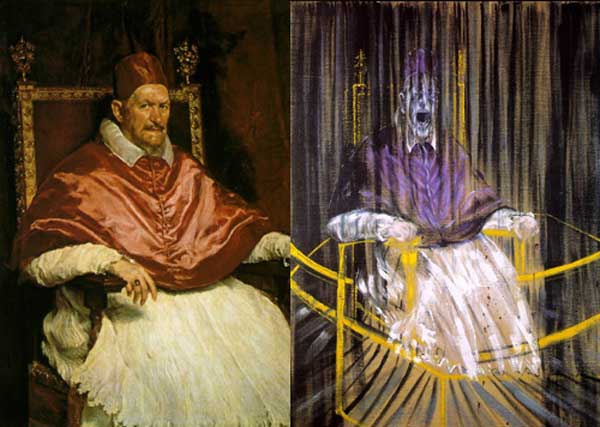
The former approaches : Francis Bacon “The Pope” (1953)
The general consensus here was that in going from $\mathbb{Z}$ to $\mathbb{F}_1$ one looses the additive structure and retains only the multiplicative one. Hence, ‘commutative algebras’ over $\mathbb{F}_1$ are (commutative) monoids, and mimicking Grothendieck’s functor of points approach to algebraic geometry, a scheme over $\mathbb{F}_1$ would then correspond to a functor
$h_Z~:~\mathbf{monoids} \longrightarrow \mathbf{sets}$
Such functors are described largely by combinatorial data (see for example the recent blueprint-paper by Oliver Lorscheid), and, if the story would stop here, any Rothko painting could be used as illustration.
Most of the former approaches add something though (buzzwords include ‘Arakelov’, ‘completion at $\infty$’, ‘real place’ etc.) in order to connect the virtual geometric object over $\mathbb{F}_1$ with existing real, complex or integral schemes. For example, one can make the virtual object visible via an evaluation map $h_Z \rightarrow h_X$ which is a natural transformation, where $X$ is a complex variety with its usual functor of points $h_X$ and to connect both we associate to a monoid $M$ its complex monoid-algebra $\mathbb{C} M$. An integral scheme $Y$ can then be said to be ‘defined over $\mathbb{F}_1$’, if $h_Z$ becomes a subfunctor of its usual functor of points $h_Y$ (again, assigning to a monoid its integral monoid algebra $\mathbb{Z} M$) and $Y$ is the ‘best’ integral scheme approximation of the complex evaluation map.
To illustrate this, consider the painting Study after Velázquez’s Portrait of Pope Innocent X by Francis Bacon (right-hand painting above) which is a distorded version of the left-hand painting Portrait of Innocent X by Diego Velázquez.
Here, Velázquez’ painting plays the role of the complex variety which makes the combinatorial gadget $h_Z$ visible, and, Bacon’s painting depicts the integral scheme, build up from this combinatorial data, which approximates the evaluation map best.
All of the former approaches more or less give the same very small list of integral schemes defined over $\mathbb{F}_1$, none of them motivically interesting.
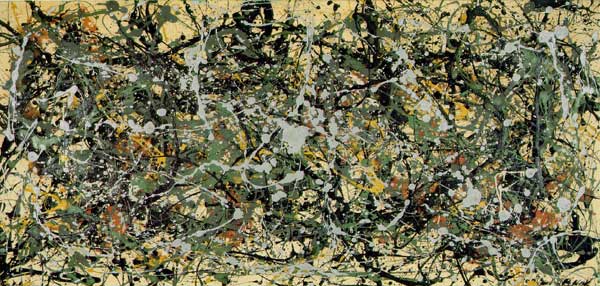
The current approach : Jackson Pollock “No. 8” (1949)
An entirely different approach was proposed by James Borger in $\Lambda$-rings and the field with one element. He proposes another definition for commutative $\mathbb{F}_1$-algebras, namely $\lambda$-rings (in the sense of Grothendieck’s Riemann-Roch) and he argues that the $\lambda$-ring structure (which amounts in the sensible cases to a family of endomorphisms of the integral ring lifting the Frobenius morphisms) can be viewed as descent data from $\mathbb{Z}$ to $\mathbb{F}_1$.
The list of integral schemes of finite type with a $\lambda$-structure coincides roughly with the list of integral schemes defined over $\mathbb{F}_1$ in the other approaches, but Borger’s theory really shines in that it proposes long sought for mystery-objects such as $\mathbf{spec}(\mathbb{Z}) \times_{\mathbf{spec}(\mathbb{F}_1)} \mathbf{spec}(\mathbb{Z})$. If one accepts Borger’s premise, then this object should be the geometric object corresponding to the Witt-ring $W(\mathbb{Z})$. Recall that the role of Witt-rings in $\mathbb{F}_1$-geometry was anticipated by Manin in Cyclotomy and analytic geometry over $\mathbb{F}_1$.
But, Witt-rings and their associated Witt-spaces are huge objects, so one needs to extend arithmetic geometry drastically to include such ‘integral schemes of infinite type’. Borger has made a couple of steps in this direction in The basic geometry of Witt vectors, II: Spaces.
To depict these new infinite dimensional geometric objects I’ve chosen for Jackson Pollock‘s painting No. 8. It is no coincidence that Pollock-paintings also appeared in the depiction of noncommutative spaces. In fact, Matilde Marcolli has made the connection between $\lambda$-rings and noncommutative geometry in Cyclotomy and endomotives by showing that the Bost-Connes endomotives are universal for $\lambda$-rings.
One Comment