Skip to content →

Tag: moonshine

Monstrous dessins 1

Dedekind’s Psi-function $\Psi(n)= n \prod_{p |n}(1 + \frac{1}{p})$ pops up in a number of topics:

  • $\Psi(n)$ is the index of the congruence subgroup $\Gamma_0(n)$ in the modular group $\Gamma=PSL_2(\mathbb{Z})$,
  • $\Psi(n)$ is the number of points in the projective line $\mathbb{P}^1(\mathbb{Z}/n\mathbb{Z})$,
  • $\Psi(n)$ is the number of classes of $2$-dimensional lattices $L_{M \frac{g}{h}}$ at hyperdistance $n$ in Conway’s big picture from the standard lattice $L_1$,
  • $\Psi(n)$ is the number of admissible maximal commuting sets of operators in the Pauli group of a single qudit.

The first and third interpretation have obvious connections with Monstrous Moonshine.

Conway’s big picture originated from the desire to better understand the Moonshine groups, and Ogg’s Jack Daniels problem
asks for a conceptual interpretation of the fact that the prime numbers such that $\Gamma_0(p)^+$ is a genus zero group are exactly the prime divisors of the order of the Monster simple group.

Here’s a nice talk by Ken Ono : Can’t you just feel the Moonshine?


For this reason it might be worthwhile to make the connection between these two concepts and the number of points of $\mathbb{P}^1(\mathbb{Z}/n\mathbb{Z})$ as explicit as possible.

Surely all of this is classical, but it is nicely summarised in the paper by Tatitscheff, He and McKay “Cusps, congruence groups and monstrous dessins”.

The ‘monstrous dessins’ from their title refers to the fact that the lattices $L_{M \frac{g}{h}}$ at hyperdistance $n$ from $L_1$ are permuted by the action of the modular groups and so determine a Grothendieck’s dessin d’enfant. In this paper they describe the dessins corresponding to the $15$ genus zero congruence subgroups $\Gamma_0(n)$, that is when $n=1,2,3,4,5,6,7,8,9,10,12,13,16,18$ or $25$.

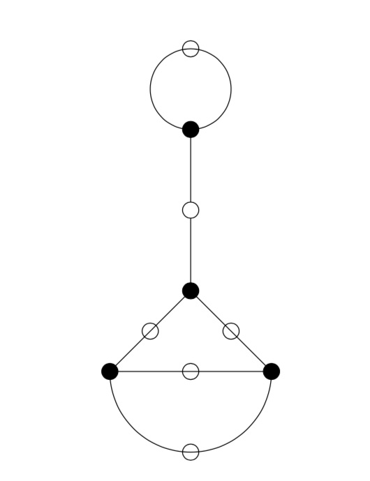
Here’s the ‘monstrous dessin’ for $\Gamma_0(6)$


But, one can compute these dessins for arbitrary $n$, describing the ripples in Conway’s big picture, and try to figure out whether they are consistent with the Riemann hypothesis.

We will get there eventually, but let’s start at an easy pace and try to describe the points of the projective line $\mathbb{P}^1(\mathbb{Z}/n \mathbb{Z})$.

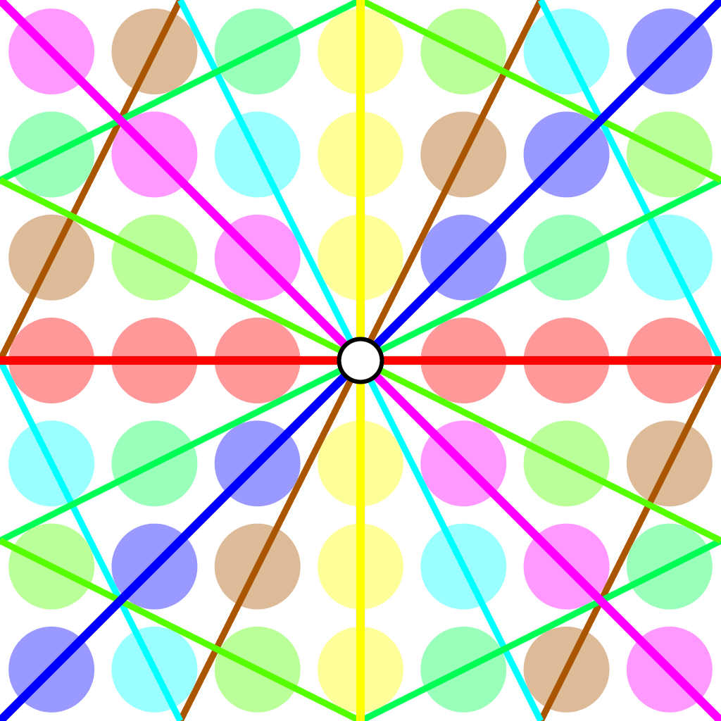
Over a field $k$ the points of $\mathbb{P}^1(k)$ correspond to the lines through the origin in the affine plane $\mathbb{A}^2(k)$ and they can represented by projective coordinates $[a:b]$ which are equivalence classes of couples $(a,b) \in k^2- \{ (0,0) \}$ under scalar multiplication with non-zero elements in $k$, so with points $[a:1]$ for all $a \in k$ together with the point at infinity $[1:0]$. When $n=p$ is a prime number we have $\# \mathbb{P}^1(\mathbb{Z}/p\mathbb{Z}) = p+1$. Here are the $8$ lines through the origin in $\mathbb{A}^2(\mathbb{Z}/7\mathbb{Z})$


Over an arbitrary (commutative) ring $R$ the points of $\mathbb{P}^1(R)$ again represent equivalence classes, this time of pairs
\[
(a,b) \in R^2~:~aR+bR=R \]
with respect to scalar multiplication by units in $R$, that is
\[
(a,b) \sim (c,d)~\quad~\text{iff}~\qquad \exists \lambda \in R^*~:~a=\lambda c, b = \lambda d \]
For $\mathbb{P}^1(\mathbb{Z}/n \mathbb{Z})$ we have to find all pairs of integers $(a,b) \in \mathbb{Z}^2$ with $0 \leq a,b < n$ with $gcd(a,b)=1$ and use Cremona’s trick to test for equivalence:
\[
(a,b) = (c,d) \in \mathbb{P}^1(\mathbb{Z}/n \mathbb{Z})~\quad \text{iff}~\quad ad-bc \equiv 0~mod~n \]
The problem is to find a canonical representative in each class in an efficient way because this is used a huge number of times in working with modular symbols.

Perhaps the best algorithm, for large $n$, is sketched in pages 145-146 of Bill Stein’s Modular forms: a computational approach.

For small $n$ the algorithm in $\S 1.3$ in the Tatitscheff, He and McKay paper suffices:

  • Consider the action of $(\mathbb{Z}/n\mathbb{Z})^*$ on $\{ 0,1,…,n-1 \}=\mathbb{Z}/n\mathbb{Z}$ and let $D$ be the set of the smallest elements in each orbit,
  • For each $d \in D$ compute the stabilizer subgroup $G_d$ for this action and let $C_d$ be the set of smallest elements in each $G_d$-orbit on the set of all elements in $\mathbb{Z}/n \mathbb{Z}$ coprime with $d$,
  • Then $\mathbb{P}^1(\mathbb{Z}/n\mathbb{Z})= \{ [c:d]~|~d \in D, c \in C_d \}$.

Let’s work this out for $n=12$ which will be our running example (the smallest non-squarefree non-primepower):

  • $(\mathbb{Z}/12\mathbb{Z})^* = \{ 1,5,7,11 \} \simeq C_2 \times C_2$,
  • The orbits on $\{ 0,1,…,11 \}$ are
    \[
    \{ 0 \}, \{ 1,5,7,11 \}, \{ 2,10 \}, \{ 3,9 \}, \{ 4,8 \}, \{ 6 \} \]
    and $D=\{ 0,1,2,3,4,6 \}$,
  • $G_0 = C_2 \times C_2$, $G_1 = \{ 1 \}$, $G_2 = \{ 1,7 \}$, $G_3 = \{ 1,5 \}$, $G_4=\{ 1,7 \}$ and $G_6=C_2 \times C_2$,
  • $1$ is the only number coprime with $0$, giving us $[1:0]$,
  • $\{ 0,1,…,11 \}$ are all coprime with $1$, and we have trivial stabilizer, giving us the points $[0:1],[1:1],…,[11:1]$,
  • $\{ 1,3,5,7,9,11 \}$ are coprime with $2$ and under the action of $\{ 1,7 \}$ they split into the orbits
    \[
    \{ 1,7 \},~\{ 3,9 \},~\{ 5,11 \} \]
    giving us the points $[1:2],[3:2]$ and $[5:2]$,
  • $\{ 1,2,4,5,7,8,10,11 \}$ are coprime with $3$, the action of $\{ 1,5 \}$ gives us the orbits
    \[
    \{ 1,5 \},~\{ 2,10 \},~\{ 4,8 \},~\{ 7,11 \} \]
    and additional points $[1:3],[2:3],[4:3]$ and $[7:3]$,
  • $\{ 1,3,5,7,9,11 \}$ are coprime with $4$ and under the action of $\{ 1,7 \}$ we get orbits
    \[
    \{ 1,7 \},~\{ 3,9 \},~\{ 5,11 \} \]
    and points $[1:4],[3:4]$ and $[5,4]$,
  • Finally, $\{ 1,5,7,11 \}$ are the only coprimes with $6$ and they form a single orbit under $C_2 \times C_2$ giving us just one additional point $[1:6]$.

This gives us all $24= \Psi(12)$ points of $\mathbb{P}^1(\mathbb{Z}/12 \mathbb{Z})$ (strangely, op page 43 of the T-H-M paper they use different representants).

One way to see that $\# \mathbb{P}^1(\mathbb{Z}/n \mathbb{Z}) = \Psi(n)$ comes from a consequence of the Chinese Remainder Theorem that for the prime factorization $n = p_1^{e_1} … p_k^{e_k}$ we have
\[
\mathbb{P}^1(\mathbb{Z}/n \mathbb{Z}) = \mathbb{P}^1(\mathbb{Z}/p_1^{e_1} \mathbb{Z}) \times … \times \mathbb{P}^1(\mathbb{Z}/p_k^{e_k} \mathbb{Z}) \]
and for a prime power $p^k$ we have canonical representants for $\mathbb{P}^1(\mathbb{Z}/p^k \mathbb{Z})$
\[
[a:1]~\text{for}~a=0,1,…,p^k-1~\quad \text{and} \quad [1:b]~\text{for}~b=0,p,2p,3p,…,p^k-p \]
which shows that $\# \mathbb{P}^1(\mathbb{Z}/p^k \mathbb{Z}) = (p+1)p^{k-1}= \Psi(p^k)$.

Next time, we’ll connect $\mathbb{P}^1(\mathbb{Z}/n \mathbb{Z})$ to Conway’s big picture and the congruence subgroup $\Gamma_0(n)$.

Leave a Comment

RH and the Ishango bone

“She simply walked into the pond in Kensington Gardens Sunday morning and drowned herself in three feet of water.”

This is the opening sentence of The Ishango Bone, a novel by Paul Hastings Wilson. It (re)tells the story of a young mathematician at Cambridge, Amiele, who (dis)proves the Riemann Hypothesis at the age of 26, is denied the Fields medal, and commits suicide.

In his review of the novel on MathFiction, Alex Kasman casts he story in the 1970ties, based on the admission of the first female students to Trinity.

More likely, the correct time frame is in the first decade of this century. On page 121 Amiele meets Alain Connes, said to be a “past winner of the Crafoord Prize”, which Alain obtained in 2001. In fact, noncommutative geometry and its interaction with quantum physics plays a crucial role in her ‘proof’.


The Ishango artefact only appears in the Coda to the book. There are a number of theories on the nature and grouping of the scorings on the bone. In one column some people recognise the numbers 11, 13, 17 and 19 (the primes between 10 and 20).

In the book, Amiele remarks that the total number of lines scored on the bone (168) “happened to be the exact total of all the primes between 1 and 1000” and “if she multiplied 60, the total number of lines in one side column, by 168, the grand total of lines, she’d get 10080,…,not such a far guess from 9592, the actual total of primes between 1 and 100000.” (page 139-140)

The bone is believed to be more than 20000 years old, prime numbers were probably not understood until about 500 BC…


More interesting than these speculations on the nature of the Ishango bone is the description of the tools Amiele thinks to need to tackle the Riemann Hypothesis:

“These included algebraic geometry (which combines commutative algebra with the language and problems of geometry); noncommutative geometry (concerned with the geometric approach to associative algebras, in which multiplication is not commutative, that is, for which $x$ times $y$ does not always equal $y$ times $x$); quantum field theory on noncommutative spacetime, and mathematical aspects of quantum models of consciousness, to name a few.” (page 115)

The breakthrough came two years later when Amiele was giving a lecture on Grothendieck’s dessins d’enfant.

“Dessin d’enfant, or ‘child’s drawing’, which Amiele had discovered in Grothendieck’s work, is a type of graph drawing that seemed technically simple, but had a very strong impression on her, partly due to the familiar nature of the objects considered. (…) Amiele found subtle arithmetic invariants associated with these dessins, which were completely transformed, again, as soon as another stroke was added.” (page 116)

Amiele’s ‘disproof’ of RH is outlined on pages 122-124 of “The Ishango Bone” and is a mixture of recognisable concepts and ill-defined terms.

“Her final result proved that Riemann’s Hypothesis was false, a zero must fall to the east of Riemann’s critical line whenever the zeta function of point $q$ with momentum $p$ approached the aelotropic state-vector (this is a simplification, of course).” (page 123)

More details are given in a footnote:

“(…) a zero must fall to the east of Riemann’s critical line whenever:

\[
\zeta(q_p) = \frac{( | \uparrow \rangle + \Psi) + \frac{1}{2}(1+cos(\Theta))\frac{\hbar}{\pi}}{\int(\Delta_p)} \]

(…) The intrepid are invited to try the equation for themselves.” (page 124)

Wilson’s “The Ishango Bone” was published in 2012. A fair number of topics covered (the Ishango bone, dessin d’enfant, Riemann hypothesis, quantum theory) also play a prominent role in the 2015 paper/story by Michel Planat “A moonshine dialogue in mathematical physics”, but this time with additional story-line: monstrous moonshine

Such a paper surely deserves a separate post.


Leave a Comment

the monster dictates her picture

The monstrous moonshine picture is a sub-graph of Conway’s Big Picture on 218 vertices. These vertices are the classes of lattices needed in the construction of the 171 moonshine groups. That is, moonshine gives us the shape of the picture.

(image credit Friendly Monsters)

But we can ask to reverse this process. Is the shape of the picture dictated by group-theoretic properties of the monster?

That is, can we reconstruct the 218 lattices and their edges starting from say the conjugacy classes of the monster and some simple rules?

Look at the the power maps for the monster. That is, the operation on conjugacy classes sending the class of $g$ to that of $g^k$ for all divisors $k$ of the order of $g$. Or, if you prefer, the $\lambda$-ring structure on the representation ring.

Rejoice die-hard believers in $\mathbb{F}_1$-theory, rejoice!

Here’s the game to play.

Let $g$ be a monster element of order $n$ and take $d=gcd(n,24)$.

(1) : If $d=8$ and a power map of $g$ gives class $8C$ add $(n|4)$ to your list.

(2) : Otherwise, look at the smallest power of $g$ such that the class is one of $12J,8F,6F,4D, 3C,2B$ or $1A$ and add $(n|e)$ where $e$ is the order of that class, or, if $n > 24$ and $e$ is even add $(n | \frac{e}{2})$.

A few examples:

For class 20E, $d=4$ and the power maps give classes 4D and 2B, so we add $(20|2)$.

For class 32B, $d=8$ but the power map gives 8E so we resort to rule (2). Here the power maps give 8E, 4C and 2B. So, the best class is 4C but as $32 > 24$ we add $(32|2)$.

For class 93A, $d=3$ and the power map gives 3C and even though $93 > 24$ we add $(93|3)$.

This gives us a list of instances $(n|e)$ with $n$ the order of a monster element. For $N=n \times e$ look at all divisors $h$ of $24$ such that $h^2$ divides $N$ and add to your list of lattices those of the form $M \frac{g}{h}$ with $g$ strictly smaller than $h$ and $(g,h)=1$ and $M$ a divisor of $\frac{N}{h^2}$.

This gives us a list of lattices $M \frac{g}{h}$, which is an $h$-th root of unity centered as $L=M \times h$ (see this post). If we do this for all lattices in the list we can partition the $L$’s in families according to which roots of unity are centered at $L$.

This gives us the moonshine picture. (modulo mistakes I made)

The operations we have to do after we have our list of instances $(n|e)$ is pretty straightforward from the rules we used to determine the lattices needed to describe a moonshine group.

Perhaps the oddest part in the construction are the rules (1) and (2) and the prescribed conjugacy classes used in them.

One way to look at this is that the classes $8C$ and $12J$ (or $24J$) are special. The other classes are just the power-maps of $12J$.

Another ‘rationale’ behind these classes may come from the notion of harmonics (see the original Monstrous moonshine paper page 312) of the identity element and the two classes of involutions, 2A (the Fischer involutions) and 2B (the Conway involutions).

For 1A these are : 1A,3C

For 2A these are : 2A,4B,8C

For 2B these are : 2B,4D,6F,8F,12J,24J

These are exactly the classes that we used in (1) and (2), if we add the power-classes of 8C.

Perhaps I should take some time to write all this down more formally.

Leave a Comment

A forgotten type and roots of unity (again)

The monstrous moonshine picture is the finite piece of Conway’s Big Picture needed to understand the 171 moonshine groups associated to conjugacy classes of the monster.

Last time I claimed that there were exactly 7 types of local behaviour, but I missed one. The forgotten type is centered at the number lattice $84$.

Locally around it the moonshine picture looks like this
\[
\xymatrix{42 \ar@{-}[dr] & 28 \frac{1}{3} \ar@[red]@{-}[d] & 41 \frac{1}{2} \ar@{-}[ld] \\ 28 \ar@[red]@{-}[r] & \color{grey}{84} \ar@[red]@{-}[r] \ar@[red]@{-}[d] \ar@{-}[rd] & 28 \frac{2}{3} \\ & 252 & 168} \]

and it involves all square roots of unity ($42$, $42 \frac{1}{2}$ and $168$) and $3$-rd roots of unity ($28$, $28 \frac{1}{3}$, $28 \frac{2}{3}$ and $252$) centered at $84$.

No, I’m not hallucinating, there are indeed $3$ square roots of unity and $4$ third roots of unity as they come in two families, depending on which of the two canonical forms to express a lattice is chosen.

In the ‘normal’ expression $M \frac{g}{h}$ the two square roots are $42$ and $42 \frac{1}{2}$ and the three third roots are $28, 28 \frac{1}{3}$ and $28 \frac{2}{3}$. But in the ‘other’ expression
\[
M \frac{g}{h} = (\frac{g’}{h},\frac{1}{h^2M}) \]
(with $g.g’ \equiv 1~mod~h$) the families of $2$-nd and $3$-rd roots of unity are
\[
\{ 42 \frac{1}{2} = (\frac{1}{2},\frac{1}{168}), 168 = (0,\frac{1}{168}) \} \]
and
\[
\{ 28 \frac{1}{3} = (\frac{1}{3},\frac{1}{252}), 28 \frac{2}{3} = (\frac{2}{3},\frac{1}{252}), 252 = (0 , \frac{1}{252}) \} \]
As in the tetrahedral snake post, it is best to view the four $3$-rd roots of unity centered at $84$ as the vertices of a tetrahedron with center of gravity at $84$. Power maps in the first family correspond to rotations along the axis through $252$ and power maps in the second family are rotations along the axis through $28$.

In the ‘normal’ expression of lattices there’s then a total of 8 different local types, but two of them consist of just one number lattice: in $8$ the local picture contains all square, $4$-th and $8$-th roots of unity centered at $8$, and in $84$ the square and $3$-rd roots.

Perhaps surprisingly, if we redo everything in the ‘other’ expression (and use the other families of roots of unity), then the moonshine picture has only 7 types of local behaviour. The forgotten type $84$ appears to split into two occurrences of other types (one with only square roots of unity, and one with only $3$-rd roots).

I wonder what all this has to do with the action of the Bost-Connes algebra on the big picture or with Plazas’ approach to moonshine via non-commutative geometry.

Leave a Comment

What we (don’t) know

Do we know why the monster exists and why there’s moonshine around it?

The answer depends on whether or not you believe that vertex operator algebras are natural, elegant and inescapable objects.

the monster

Simple groups often arise from symmetries of exceptionally nice mathematical objects.

The smallest of them all, $A_5$, gives us the rotation symmetries of the icosahedron. The next one, Klein’s simple group $L_2(7)$, comes from the Klein quartic.

The smallest sporadic groups, the Mathieu groups, come from Steiner systems, and the Conway groups from the 24-dimensional Leech lattice.

What about the largest sporadic simple, the monster $\mathbb{M}$?

In his paper What is … the monster? Richard Borcherds writes (among other characterisations of $\mathbb{M}$):

“3. It is the automorphism group of the monster vertex algebra. (This is probably the best answer.)”

But, even Borcherds adds:

“Unfortunately none of these definitions is completely satisfactory. At the moment all constructions of the algebraic structures above seem artificial; they are constructed as sums of two or more apparently unrelated spaces, and it takes a lot of effort to define the algebraic structure on the sum of these spaces and to check that the monster acts on the resulting structure.
It is still an open problem to find a really simple and natural construction of the monster vertex algebra.

Here’s 2 minutes of John Conway on the “one thing” he really wants to know before he dies: why the monster group exists.


moonshine

Moonshine started off with McKay’s observation that 196884 (the first coefficient in the normalized j-function) is the sum 1+196883 of the dimensions of the two smallest simple representations of $\mathbb{M}$.

Soon it was realised that every conjugacy class of the monster has a genus zero group (or ‘moonshine group’) associated to it.

Borcherds proved the ‘monstrous moonshine conjectures’ asserting that the associated main modular function of such a group is the character series of the action of the element on the monster vertex algebra.

Here’s Borcherds’ ICM talk in Berlin on this: What is … Moonshine?.

Once again, the monster vertex algebra appears to be the final answer.

However, in characterising the 171 moonshine groups among all possible genus zero groups one has proved that they are all of the form:

(ii) : $(n|h)+e,g,\dots$

In his book Moonshine beyond the Monster, Terry Gannon writes:

“We now understand the significance, in the VOA or CFT framework, of transformations in $SL_2(\mathbb{Z})$, but (ii) emphasises that many modular transformations relevant to Moonshine are more general (called the Atkin-Lehner involutions).
Monstrous moonshine will remain mysterious until we can understand its Atkin-Lehner symmetries.

Leave a Comment

the moonshine picture – at last

The monstrous moonshine picture is the subgraph of Conway’s big picture consisting of all lattices needed to describe the 171 moonshine groups.

It consists of:

– exactly 218 vertices (that is, lattices), out of which

– 97 are number-lattices (that is of the form $M$ with $M$ a positive integer), and

– 121 are proper number-like lattices (that is of the form $M \frac{g}{h}$ with $M$ a positive integer, $h$ a divisor of $24$ and $1 \leq g \leq h$ with $(g,h)=1$).

The $97$ number lattices are closed under taking divisors, and the corresponding Hasse diagram has the following shape

Here, number-lattices have the same colour if they have the same local structure in the moonshine picture (that is, have a similar neighbourhood of proper number-like lattices).

There are 7 different types of local behaviour:

The white numbered lattices have no proper number-like neighbours in the picture.

The yellow number lattices (2,10,14,18,22,26,32,34,40,68,80,88,90,112,126,144,180,208 = 2M) have local structure

\[
\xymatrix{M \ar@{-}[r] & \color{yellow}{2M} \ar@{-}[r] & M \frac{1}{2}} \]

which involves all $2$-nd (square) roots of unity centered at the lattice.

The green number lattices (3,15,21,39,57,93,96,120 = 3M) have local structure

\[
\xymatrix{& M \ar@[red]@{-}[d] & \\ M \frac{1}{3} \ar@[red]@{-}[r] & \color{green}{3M} \ar@[red]@{-}[r] & M \frac{2}{3}} \]

which involve all $3$-rd roots of unity centered at the lattice.

The blue number lattices (4,16,20,28,36,44,52,56,72,104 = 4M) have as local structure

\[
\xymatrix{M \frac{1}{2} \ar@{-}[d] & & M \frac{1}{4} \ar@{-}[d] \\
2M \ar@{-}[r] & \color{blue}{4M} \ar@{-}[r] & 2M \frac{1}{2} \ar@{-}[d] \\
M \ar@{-}[u] & & M \frac{3}{4}} \]

and involve the $2$-nd and $4$-th root of unity centered at the lattice.

The purple number lattices (6,30,42,48,60 = 6M) have local structure

\[
\xymatrix{& M \frac{1}{3} \ar@[red]@{-}[d] & 2M \frac{1}{3} & M \frac{1}{6} \ar@[red]@{-}[d] & \\
M \ar@[red]@{-}[r] & 3M \ar@{-}[r] \ar@[red]@{-}[d] & \color{purple}{6M} \ar@{-}[r] \ar@[red]@{-}[u] \ar@[red]@{-}[d] & 3M \frac{1}{2} \ar@[red]@{-}[r] \ar@[red]@{-}[d] & M \frac{5}{6} \\
& M \frac{2}{3} & 2M \frac{2}{3} & M \frac{1}{2} & } \]

and involve all $2$-nd, $3$-rd and $6$-th roots of unity centered at the lattice.

The unique brown number lattice 8 has local structure

\[
\xymatrix{& & 1 \frac{1}{4} \ar@{-}[d] & & 1 \frac{1}{8} \ar@{-}[d] & \\
& 1 \frac{1}{2} \ar@{-}[d] & 2 \frac{1}{2} \ar@{-}[r] \ar@{-}[d] & 1 \frac{3}{4} & 2 \frac{1}{4} \ar@{-}[r] & 1 \frac{5}{8} \\
1 \ar@{-}[r] & 2 \ar@{-}[r] & 4 \ar@{-}[r] & \color{brown}{8} \ar@{-}[r] & 4 \frac{1}{2} \ar@{-}[d] \ar@{-}[u] & \\
& & & 1 \frac{7}{8} \ar@{-}[r] & 2 \frac{3}{4} \ar@{-}[r] & 1 \frac{3}{8}} \]

which involves all $2$-nd, $4$-th and $8$-th roots of unity centered at $8$.

Finally, the local structure for the central red lattices $12,24 = 12M$ is

\[
\xymatrix{
M \frac{1}{12} \ar@[red]@{-}[dr] & M \frac{5}{12} \ar@[red]@{-}[d] & M \frac{3}{4} \ar@[red]@{-}[dl] & & M \frac{1}{6} \ar@[red]@{-}[dr] & M \frac{1}{2} \ar@[red]@{-}[d] & M \frac{5}{6} \ar@[red]@{-}[dl] \\
& 3M \frac{1}{4} \ar@{-}[dr] & 2M \frac{1}{6} \ar@[red]@{-}[d] & 4M \frac{1}{3} \ar@[red]@{-}[d] & 2M \frac{1}{3} \ar@[red]@{-}[d] & 3M \frac{1}{2} \ar@{-}[dl] & \\
& 2M \frac{1}{2} \ar@[red]@{-}[r] & 6M \frac{1}{2} \ar@{-}[dl] \ar@[red]@{-}[d] \ar@{-}[r] & \color{red}{12M} \ar@[red]@{-}[d] \ar@{-}[r] & 6M \ar@[red]@{-}[d] \ar@{-}[dr] \ar@[red]@{-}[r] & 2M & \\
& 3M \frac{3}{4} \ar@[red]@{-}[dl] \ar@[red]@{-}[d] \ar@[red]@{-}[dr] & 2M \frac{5}{6} & 4M \frac{2}{3} & 2M \frac{2}{3} & 3M \ar@[red]@{-}[dl] \ar@[red]@{-}[d] \ar@[red]@{-}[dr] & \\
M \frac{1}{4} & M \frac{7}{12} & M \frac{11}{12} & & M \frac{1}{3} & M \frac{2}{3} & M}
\]

It involves all $2$-nd, $3$-rd, $4$-th, $6$-th and $12$-th roots of unity with center $12M$.

No doubt this will be relevant in connecting moonshine with non-commutative geometry and issues of replicability as in Plazas’ paper Noncommutative Geometry of Groups like $\Gamma_0(N)$.

Another of my pet follow-up projects is to determine whether or not the monster group $\mathbb{M}$ dictates the shape of the moonshine picture.

That is, can one recover the 97 number lattices and their partition in 7 families starting from the set of element orders of $\mathbb{M}$, applying some set of simple rules?

One of these rules will follow from the two equivalent notations for lattices, and the two different sets of roots of unities centered at a given lattice. This will imply that if a number lattice belongs to a given family, certain divisors and multiples of it must belong to related families.

If this works out, it may be a first step towards a possibly new understanding of moonshine.

Leave a Comment

the monstrous moonshine picture – 2

Time to wrap up my calculations on the moonshine picture, which is the subgraph of Conway’s Big Picture needed to describe all 171 moonshine groups.

No doubt I’ve made mistakes. All corrections are welcome. The starting point is the list of 171 moonshine groups which are in the original Monstrous Moonshine paper.

The backbone is given by the $97$ number lattices, which are closed under taking divisors and were found by looking at all divisors of the numbers $N=n \times h$ for the 171 moonshine groups of the form $N+e,f,\dots$ or $(n|h)+e,f,\dots$.

The Hasse-diagram of this poset (under division) is here (click on the image to get a larger version)

There are seven types of coloured numbers, each corresponding to number-lattices which have the same local structure in the moonshine picture, as in the previous post.

The white numbered lattices have no further edges in the picture.

The yellow number lattices (2,10,14,18,22,26,32,34,40,68,80,88,90,112,126,144,180,208 = 2M) have local structure

\[
\xymatrix{& \color{yellow}{2M} \ar@{-}[r] & M \frac{1}{2}} \]

The green number lattices (3,15,21,39,57,93,96,120 = 3M) have local structure

\[
\xymatrix{M \frac{1}{3} \ar@[red]@{-}[r] & \color{green}{3M} \ar@[red]@{-}[r] & M \frac{2}{3}} \]

The blue number lattices (4,16,20,28,36,44,52,56,72,104 = 4M) have as local structure

\[
\xymatrix{M \frac{1}{2} \ar@{-}[d] & & M \frac{1}{4} \ar@{-}[d] \\
2M \ar@{-}[r] & \color{blue}{4M} \ar@{-}[r] & 2M \frac{1}{2} \ar@{-}[d] \\
& & M \frac{3}{4}} \]

where the leftmost part is redundant as they are already included in the yellow-bit.

The purple number lattices (6,30,42,48,60 = 6M) have local structure

\[
\xymatrix{M \frac{1}{3} \ar@[red]@{-}[d] & 2M \frac{1}{3} & M \frac{1}{6} \ar@[red]@{-}[d] & \\
3M \ar@{-}[r] \ar@[red]@{-}[d] & \color{purple}{6M} \ar@{-}[r] \ar@[red]@{-}[u] \ar@[red]@{-}[d] & 3M \frac{1}{2} \ar@[red]@{-}[r] \ar@[red]@{-}[d] & M \frac{5}{6} \\
M \frac{2}{3} & 2M \frac{2}{3} & M \frac{1}{2} & } \]

where again the lefmost part is redundant, and I forgot to add the central part in the previous post… (updated now).

The unique brown number lattice 8 has local structure

\[
\xymatrix{& & 1 \frac{1}{4} \ar@{-}[d] & & 1 \frac{1}{8} \ar@{-}[d] & \\
& 1 \frac{1}{2} \ar@{-}[d] & 2 \frac{1}{2} \ar@{-}[r] \ar@{-}[d] & 1 \frac{3}{4} & 2 \frac{1}{4} \ar@{-}[r] & 1 \frac{5}{8} \\
1 \ar@{-}[r] & 2 \ar@{-}[r] & 4 \ar@{-}[r] & \color{brown}{8} \ar@{-}[r] & 4 \frac{1}{2} \ar@{-}[d] \ar@{-}[u] & \\
& & & 1 \frac{7}{8} \ar@{-}[r] & 2 \frac{3}{4} \ar@{-}[r] & 1 \frac{3}{8}} \]

The local structure in the two central red number lattices (not surprisingly 12 and 24) looks like the image in the previous post, but I have to add some ‘forgotten’ lattices.

That’ll have to wait…

Leave a Comment

Moonshine’s green anaconda

The largest snake in the moonshine picture determines the moonshine group $(24|12)$ and is associated to conjugacy class $24J$ of the monster.

It contains $70$ lattices, about one third of the total number of lattices in the moonshine picture.

The anaconda’s backbone is the $(288|1)$ thread below (edges in the $2$-tree are black, those in the $3$-tree red and coloured numbers are symmetric with respect to the $(24|12)$-spine and have the same local snake-structure.

\[
\xymatrix{9 \ar@{-}[r] \ar@[red]@{-}[d] & \color{green}{18} \ar@{-}[r] \ar@[red]@{-}[d] & \color{yellow}{36} \ar@{-}[r] \ar@[red]@{-}[d] & \color{yellow}{72} \ar@{-}[r] \ar@[red]@{-}[d] & \color{green}{144} \ar@{-}[r] \ar@[red]@{-}[d] & 288 \ar@[red]@{-}[d] \\
3 \ar@{-}[r] \ar@[red]@{-}[d] & \color{blue}{6} \ar@{-}[r] \ar@[red]@{-}[d] & \color{red}{12} \ar@{-}[r] \ar@[red]@{-}[d] & \color{red}{24} \ar@{-}[r] \ar@[red]@{-}[d] & \color{blue}{48} \ar@{-}[r] \ar@[red]@{-}[d] & 96 \ar@[red]@{-}[d] \\
1 \ar@{-}[r] & \color{green}{2} \ar@{-}[r] & \color{yellow}{4} \ar@{-}[r] & \color{yellow}{8} \ar@{-}[r] & \color{green}{16} \ar@{-}[r] & 32 } \]

These are the only number-lattices in the anaconda. The remaining lattices are number-like, that is of the form $M \frac{g}{h}$ with $M$ an integer and $1 \leq g < h$ with $(g,h)=1$.
There are

– $12$ with $h=2$ and $M$ a divisor of $72$.

– $12$ with $h=3$ and $M$ a divisor of $32$.

– $12$ with $h=4$ and $M$ a divisor of $18$.

– $8$ with $h=6$ and $M$ a divisor of $8$.

– $8$ with $h=12$ and $M=1,2$.

The non-number lattices in the snake are locally in the coloured numbers:

In $2,16,18,144=2M$

\[
\xymatrix{& \color{green}{2M} \ar@{-}[r] & M \frac{1}{2}} \]

In $4,8,36,72=4M$

\[
\xymatrix{M \frac{1}{2} \ar@{-}[d] & & M \frac{1}{4} \ar@{-}[d] \\
2M \ar@{-}[r] & \color{yellow}{4M} \ar@{-}[r] & 2M \frac{1}{2} \ar@{-}[d] \\
& & M \frac{3}{4}} \]

In $6,48=6M$

\[
\xymatrix{M \frac{1}{3} \ar@[red]@{-}[d] & 2M \frac{1}{3} & M \frac{1}{6} \ar@[red]@{-}[d] & \\
3M \ar@{-}[r] \ar@[red]@{-}[d] & \color{blue}{6M} \ar@{-}[r] \ar@[red]@{-}[u] \ar@[red]@{-}[d] & 3M \frac{1}{2} \ar@[red]@{-}[r] \ar@[red]@{-}[d] & M \frac{5}{6} \\
M \frac{2}{3} & 2M \frac{2}{3} & M \frac{1}{2} & } \]

In $12,24=12M$ the local structure looks like

Here, we used the commutation relations to reach all lattices at distance $log(6)$ and $log(12)$ by first walking the $2$-adic tree and postpone the last step for the $3$-tree.

Perhaps this is also a good strategy to get a grip on the full moonshine picture:

First determine subsets of the moonshine thread with the same local structure, and then determine for each class this local structure.

Leave a Comment

the 171 moonshine groups

Monstrous moonshine associates to every element of order $n$ of the monster group $\mathbb{M}$ an arithmetic group of the form
\[
(n|h)+e,f,\dots \]
where $h$ is a divisor of $24$ and of $n$ and where $e,f,\dots$ are divisors of $\frac{n}{h}$ coprime with its quotient.

In snakes, spines, and all that we’ve constructed the arithmetic group
\[
\Gamma_0(n|h)+e,f,\dots \]
which normalizes $\Gamma_0(N)$ for $N=h.n$. If $h=1$ then this group is the moonshine group $(n|h)+e,f,\dots$, but for $h > 1$ the moonshine group is a specific subgroup of index $h$ in $\Gamma_0(n|h)+e,f,\dots$.

I’m sure one can describe this subgroup explicitly in each case by analysing the action of the finite group $(\Gamma_0(n|h)+e,f,\dots)/\Gamma_0(N)$ on the $(N|1)$-snake. Some examples were worked out by John Duncan in his paper Arithmetic groups and the affine E8 Dynkin diagram.

But at the moment I don’t understand the general construction given by Conway, McKay and Sebbar in On the discrete groups of moonshine. I’m stuck at the last sentence of (2) in section 3. Nothing a copy of Charles Ferenbaugh Ph. D. thesis cannot fix.

The correspondence between the conjugacy classes of the Monster and these arithmetic groups takes up 3 pages in Conway & Norton’s Monstrous Moonshine. Here’s the beginning of it.

Leave a Comment

Snakes, spines, threads and all that

Conway introduced his Big Picture to make it easier to understand and name the groups appearing in Monstrous Moonshine.

For $M \in \mathbb{Q}_+$ and $0 \leq \frac{g}{h} < 1$, $M,\frac{g}{h}$ denotes (the projective equivalence class of) the lattice \[ \mathbb{Z} (M \vec{e}_1 + \frac{g}{h} \vec{e}_2) \oplus \mathbb{Z} \vec{e}_2 \] which we also like to represent by the $2 \times 2$ matrix \[ \alpha_{M,\frac{g}{h}} = \begin{bmatrix} M & \frac{g}{h} \\ 0 & 1 \end{bmatrix} \] A subgroup $G$ of $GL_2(\mathbb{Q})$ is said to fix $M,\frac{g}{h}$ if
\[
\alpha_{M,\frac{g}{h}}.G.\alpha_{M,\frac{g}{h}}^{-1} \subset SL_2(\mathbb{Z}) \]
The full group of all elements fixing $M,\frac{g}{h}$ is the conjugate
\[
\alpha_{M,\frac{g}{h}}^{-1}.SL_2(\mathbb{Z}).\alpha_{M,\frac{g}{h}} \]
For a number lattice $N=N,0$ the elements of this group are all of the form
\[
\begin{bmatrix} a & \frac{b}{N} \\ cN & d \end{bmatrix} \qquad \text{with} \qquad \begin{bmatrix} a & b \\ c & d \end{bmatrix} \in SL_2(\mathbb{Z}) \]
and the intersection with $SL_2(\mathbb{Z})$ (which is the group of all elements fixing the lattice $1=1,0$) is the congruence subgroup
\[
\Gamma_0(N) = \{ \begin{bmatrix} a & b \\ cN & d \end{bmatrix}~|~ad-Nbc = 1 \} \]
Conway argues that this is the real way to think of $\Gamma_0(N)$, as the joint stabilizer of the two lattices $N$ and $1$!

The defining definition of 24 tells us that $\Gamma_0(N)$ fixes more lattices. In fact, it fixes exactly the latices $M \frac{g}{h}$ such that
\[
1~|~M~|~\frac{N}{h^2} \quad \text{with} \quad h^2~|~N \quad \text{and} \quad h~|~24 \]
Conway calls the sub-graph of the Big Picture on these lattices the snake of $(N|1)$.

Here’s the $(60|1)$-snake (note that $60=2^2.3.5$ so $h=1$ or $h=2$ and edges corresponding to the prime $2$ are coloured red, those for $3$ green and for $5$ blue).

\[
\xymatrix{& & & 15 \frac{1}{2} \ar@[red]@{-}[dd] & & \\
& & 5 \frac{1}{2} \ar@[red]@{-}[dd] & & & \\
& 15 \ar@[red]@{-}[rr] \ar@[blue]@{-}[dd] & & 30 \ar@[red]@{-}[rr] \ar@[blue]@{-}[dd] & & 60 \ar@[blue]@{-}[dd] \\
5 \ar@[green]@{-}[ru] \ar@[blue]@{-}[dd] \ar@[red]@{-}[rr] & & 10 \ar@[green]@{-}[ru] \ar@[red]@{-}[rr] \ar@[blue]@{-}[dd] & & 20 \ar@[green]@{-}[ru] \ar@[blue]@{-}[dd] & \\
& 3 \ar@[red]@{-}[rr] & & 6 \ar@[red]@{-}[rr] \ar@[red]@{-}[dd] & & 12 \\
1 \ar@[green]@{-}[ru] \ar@[red]@{-}[rr] & & 2 \ar@[green]@{-}[ru] \ar@[red]@{-}[rr] \ar@[red]@{-}[dd] & & 4 \ar@[green]@{-}[ru] & \\
& & & 3\frac{1}{2} & & \\
& & 1 \frac{1}{2} & & &} \]

The sub-graph of lattices fixed by $\Gamma_0(N)$ for $h=1$, that is all number-lattices $M=M,0$ for $M$ a divisor of $N$ is called the thread of $(N|1)$. Here’s the $(60|1)$-thread

\[
\xymatrix{
& 15 \ar@[red]@{-}[rr] \ar@[blue]@{-}[dd] & & 30 \ar@[red]@{-}[rr] \ar@[blue]@{-}[dd] & & 60 \ar@[blue]@{-}[dd] \\
5 \ar@[green]@{-}[ru] \ar@[blue]@{-}[dd] \ar@[red]@{-}[rr] & & 10 \ar@[green]@{-}[ru] \ar@[red]@{-}[rr] \ar@[blue]@{-}[dd] & & 20 \ar@[green]@{-}[ru] \ar@[blue]@{-}[dd] & \\
& 3 \ar@[red]@{-}[rr] & & 6 \ar@[red]@{-}[rr] & & 12 \\
1 \ar@[green]@{-}[ru] \ar@[red]@{-}[rr] & & 2 \ar@[green]@{-}[ru] \ar@[red]@{-}[rr] & & 4 \ar@[green]@{-}[ru] &
} \]

If $N$ factors as $N = p_1^{e_1} p_2^{e_2} \dots p_k^{e_k}$ then the $(N|1)$-thread is the product of the $(p_i^{e_i}|1)$-threads and has a symmetry group of order $2^k$.

It is generated by $k$ involutions, each one the reflexion in one $(p_i^{e_i}|1)$-thread and the identity on the other $(p_j^{e_j}|1)$-threads.
In the $(60|1)$-thread these are the reflexions in the three mirrors of the figure.

So, there is one involution for every divisor $e$ of $N$ such that $(e,\frac{N}{e})=1$. For such an $e$ there are matrices, with $a,b,c,d \in \mathbb{Z}$, of the form
\[
W_e = \begin{bmatrix} ae & b \\ cN & de \end{bmatrix} \quad \text{with} \quad ade^2-bcN=e \]
Think of Bezout and use that $(e,\frac{N}{e})=1$.

Such $W_e$ normalizes $\Gamma_0(N)$, that is, for any $A \in \Gamma_0(N)$ we have that $W_e.A.W_e^{-1} \in \Gamma_0(N)$. Also, the determinant of $W_e^e$ is equal to $e^2$ so we can write $W_e^2 = e A$ for some $A \in \Gamma_0(N)$.

That is, the transformation $W_e$ (left-multiplication) sends any lattice in the thread or snake of $(N|1)$ to another such lattice (up to projective equivalence) and if we apply $W_e^2$ if fixes each such lattice (again, up to projective equivalence), so it is the desired reflexion corresponding with $e$.

Consider the subgroup of $GL_2(\mathbb{Q})$ generated by $\Gamma_0(N)$ and some of these matrices $W_e,W_f,\dots$ and denote by $\Gamma_0(N)+e,f,\dots$ the quotient modulo positive scalar matrices, then
\[
\Gamma_0(N) \qquad \text{is a normal subgroup of} \qquad \Gamma_0(N)+e,f,\dots \]
with quotient isomorphic to some $(\mathbb{Z}/2\mathbb{Z})^l$ isomorphic to the subgroup generated by the involutions corresponding to $e,f,\dots$.

More generally, consider the $(n|h)$-thread for number lattices $n=n,0$ and $h=h,0$ such that $h | n$ as the sub-graph on all number lattices $l=l,0$ such that $h | l | n$. If we denote with $\Gamma_0(n|h)$ the point-wise stabilizer of $n$ and $h$, then we have that
\[
\Gamma(n|h) = \begin{bmatrix} h & 0 \\ 0 & 1 \end{bmatrix}^{-1}.\Gamma_0(\frac{n}{h}).\begin{bmatrix} h & 0 \\ 0 & 1 \end{bmatrix} \]
and we can then denote with
\[
\Gamma_0(n|h)+e,f,\dots \]
the conjugate of the corresponding group $\Gamma_0(\frac{n}{h})+e,f,\dots$.

If $h$ is the largest divisor of $24$ such that $h^2$ divides $N$, then Conway calls the spine of the $(N|1)$-snake the subgraph on all lattices of the snake whose distance from its periphery is exactly $log(h)$.

For $N=60$, $h=2$ and so the spine of the $(60|1)$-snake is the central piece connected with double black edges

\[
\xymatrix{& & & 15 \frac{1}{2} \ar@[red]@{-}[dd] & & \\
& & 5 \frac{1}{2} \ar@[red]@{-}[dd] & & & \\
& 15 \ar@[red]@{-}[rr] \ar@[blue]@{-}[dd] & & 30 \ar@[red]@{-}[rr] \ar@[black]@{=}[dd] & & 60 \ar@[blue]@{-}[dd] \\
5 \ar@[green]@{-}[ru] \ar@[blue]@{-}[dd] \ar@[red]@{-}[rr] & & 10 \ar@[black]@{=}[ru] \ar@[red]@{-}[rr] \ar@[black]@{=}[dd] & & 20 \ar@[green]@{-}[ru] \ar@[blue]@{-}[dd] & \\
& 3 \ar@[red]@{-}[rr] & & 6 \ar@[red]@{-}[rr] \ar@[red]@{-}[dd] & & 12 \\
1 \ar@[green]@{-}[ru] \ar@[red]@{-}[rr] & & 2 \ar@[black]@{=}[ru] \ar@[red]@{-}[rr] \ar@[red]@{-}[dd] & & 4 \ar@[green]@{-}[ru] & \\
& & & 3\frac{1}{2} & & \\
& & 1 \frac{1}{2} & & &} \]

which is the $(30|2)$-thread.

The upshot of all this is to have a visual proof of the Atkin-Lehner theorem which says that the full normalizer of $\Gamma_0(N)$ is the group $\Gamma_0(\frac{N}{h}|h)+$ (that is, adding all involutions) where $h$ is the largest divisor of $24$ for which $h^2|N$.

Any element of this normalizer must take every lattice in the $(N|1)$-snake fixed by $\Gamma_0(N)$ to another such lattice. Thus it follows that it must take the snake to itself.
Conversely, an element that takes the snake to itself must conjugate into itself the group of all matrices that fix every point of the snake, that is to say, must normalize $\Gamma_0(N)$.

But the elements that take the snake to itself are precisely those that take the spine to itself, and since this spine is just the $(\frac{N}{h}|h)$-thread, this group is just $\Gamma_0(\frac{N}{h}|h)+$.

Reference: J.H. Conway, “Understanding groups like $\Gamma_0(N)$”, in “Groups, Difference Sets, and the Monster”, Walter de Gruyter-Berlin-New York, 1996

Leave a Comment