“She simply walked into the pond in Kensington Gardens Sunday morning and drowned herself in three feet of water.”
This is the opening sentence of The Ishango Bone, a novel by Paul Hastings Wilson. It (re)tells the story of a young mathematician at Cambridge, Amiele, who (dis)proves the Riemann Hypothesis at the age of 26, is denied the Fields medal, and commits suicide.
In his review of the novel on MathFiction, Alex Kasman casts he story in the 1970ties, based on the admission of the first female students to Trinity.
More likely, the correct time frame is in the first decade of this century. On page 121 Amiele meets Alain Connes, said to be a “past winner of the Crafoord Prize”, which Alain obtained in 2001. In fact, noncommutative geometry and its interaction with quantum physics plays a crucial role in her ‘proof’.
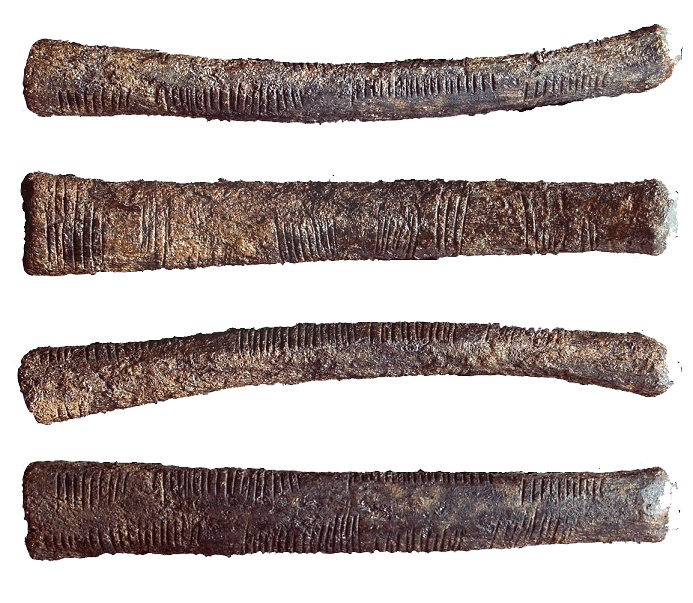
The Ishango artefact only appears in the Coda to the book. There are a number of theories on the nature and grouping of the scorings on the bone. In one column some people recognise the numbers 11, 13, 17 and 19 (the primes between 10 and 20).
In the book, Amiele remarks that the total number of lines scored on the bone (168) “happened to be the exact total of all the primes between 1 and 1000” and “if she multiplied 60, the total number of lines in one side column, by 168, the grand total of lines, she’d get 10080,…,not such a far guess from 9592, the actual total of primes between 1 and 100000.” (page 139-140)
The bone is believed to be more than 20000 years old, prime numbers were probably not understood until about 500 BC…
More interesting than these speculations on the nature of the Ishango bone is the description of the tools Amiele thinks to need to tackle the Riemann Hypothesis:
“These included algebraic geometry (which combines commutative algebra with the language and problems of geometry); noncommutative geometry (concerned with the geometric approach to associative algebras, in which multiplication is not commutative, that is, for which $x$ times $y$ does not always equal $y$ times $x$); quantum field theory on noncommutative spacetime, and mathematical aspects of quantum models of consciousness, to name a few.” (page 115)
The breakthrough came two years later when Amiele was giving a lecture on Grothendieck’s dessins d’enfant.
“Dessin d’enfant, or ‘child’s drawing’, which Amiele had discovered in Grothendieck’s work, is a type of graph drawing that seemed technically simple, but had a very strong impression on her, partly due to the familiar nature of the objects considered. (…) Amiele found subtle arithmetic invariants associated with these dessins, which were completely transformed, again, as soon as another stroke was added.” (page 116)
Amiele’s ‘disproof’ of RH is outlined on pages 122-124 of “The Ishango Bone” and is a mixture of recognisable concepts and ill-defined terms.
“Her final result proved that Riemann’s Hypothesis was false, a zero must fall to the east of Riemann’s critical line whenever the zeta function of point $q$ with momentum $p$ approached the aelotropic state-vector (this is a simplification, of course).” (page 123)
More details are given in a footnote:
“(…) a zero must fall to the east of Riemann’s critical line whenever:
\[
\zeta(q_p) = \frac{( | \uparrow \rangle + \Psi) + \frac{1}{2}(1+cos(\Theta))\frac{\hbar}{\pi}}{\int(\Delta_p)} \]
(…) The intrepid are invited to try the equation for themselves.” (page 124)
Wilson’s “The Ishango Bone” was published in 2012. A fair number of topics covered (the Ishango bone, dessin d’enfant, Riemann hypothesis, quantum theory) also play a prominent role in the 2015 paper/story by Michel Planat “A moonshine dialogue in mathematical physics”, but this time with additional story-line: monstrous moonshine…
Such a paper surely deserves a separate post.