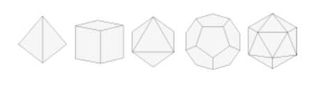
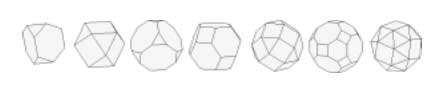
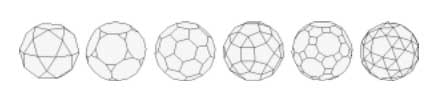
We are after the geometric trinity corresponding to the trinity of exceptional Galois groups
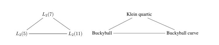
The surfaces on the right have the corresponding group on the left as their group of automorphisms. But, there is a lot more group-theoretic info hidden in the geometry. Before we sketch the $L_2(11) $ case, let us recall the simpler situation of $L_2(7) $.
There are some excellent web-page on the Klein quartic and it would be too hard to try to improve on them, so we refer to John Baez’ page and Greg Egan’s page for more details.
The Klein quartic is the degree 4 projective plane curve defined by the equation $x^3y+y^3z+z^3x=0 $. It can be tiled with a set of 24 regular heptagons, or alternatively with a set of 56 equilateral triangles and these two tilings are dual to each other

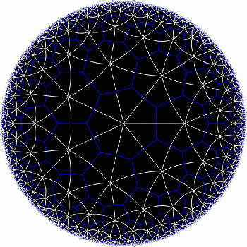
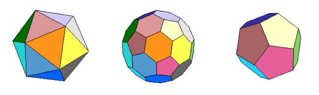
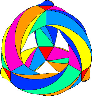
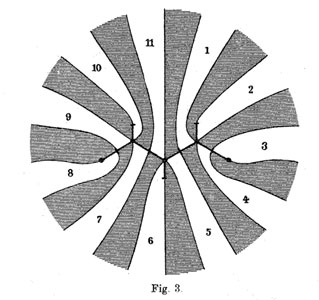
In the triangular tiling, there are 56 triangles, 84 edges and 24 vertices. The 56 triangles come in 7 bunches of 8 each and we give the 7 bunches of triangles each a different color as in the pictures below made by Greg Egan. Observe that in the hyperbolic tiling all triangles look alike, but in the picture on the left most of them get warped as we try to embed the quartic in 3-space (which is impossible to do properly). The non-warped triangles (the red ones) come into pairs, the top and bottom triangles of a triangular prism, one prism at each of the four ‘vertices’ of a tetrahedron.
The automorphism group $L_2(7) $ acts on these triangles as $S_4 $ acts on the triangles in a truncated cube.
The buckyball construction from a conjugacy class of order 11 elements from $L_2(11) $ recalled last time, has an analogon $L_2(7) $, leading to the truncated cube.
In $L_2(7) $ there are two conjugacy classes of subgroups isomorphic to $S_4 $ (the rotation-symmetry group of the cube) as well as two conjugacy classes of order 7 elements, each consisting of precisely 24 elements, say C and D. The normalizer subgroup of C has order 21, so there is a cyclic group of order 3 acting non-trivially on the conjugacy class C with 8 orbits consisting of three elements each. These are the eight triangles of the truncated cube identified above as the red triangles.
 Shifting perspective, we can repeat this for each of the seven different colors. That is, we have seven truncated cubes in the Klein quartic. On each of them a copy of $S_4 $ acts and these subgroups form one of the two conjugacy classes of $S_4 $ in the group $L_2(7) $. The colors of the triangles of these seven truncated cubes are indicated by bullets in the picture above on the right. The other conjugacy class of $S_4 $’s act on ‘truncated anti-cubes’ which also come in seven bunches of which the color is indicated by a square in that picture.
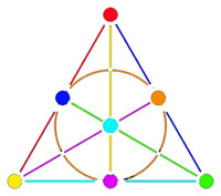
If you spend enough time on it you will see that each (truncated) cube is completely disjoint from precisely 3 (truncated) anti-cubes. This reminds us of the Fano-plane (picture on the left) : it has 7 points (our seven truncated cubes), 7 lines (the truncated anti-cubes) and the incidence relation of points and lines corresponds to the disjointness of (truncated) cubes and anti-cubes! This is the geometric interpretation of the group-theoretic realization that $L_2(7) \simeq PGL_3(\mathbb{F}_2) $ is the isomorphism group of the projective plane over the finite field $\mathbb{F}_2 $ on two elements, that is, the Fano plane. The colors of the picture on the left indicate the colors of cubes (points) and anti-cubes (lines) consistent with Egan’s picture above.
Further, the 24 vertices correspond to the 24 cusps of the modular group $\Gamma(7) $. Recall that a modular interpretation of the Klein quartic is as $\mathbb{H}/\Gamma(7) $ where $\mathbb{H} $ is the upper half-plane on which the modular group $\Gamma = PSL_2(\mathbb{Z}) $ acts via Moebius transformations, that is, to a 2×2 matrix corresponds the transformation
[tex]\begin{bmatrix} a & b \\ c & d \end{bmatrix}[/tex] <----> $ z \mapsto \frac{az+b}{cz+d} $
Okay, now let’s briefly sketch the exciting results found by Pablo Martin and David Singerman in the paper From biplanes to the Klein quartic and the buckyball, extending the above to the group $L_2(11) $.
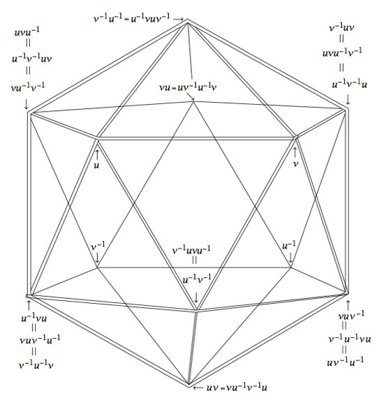
There is one important modification to be made. Recall that the Cayley-graph to get the truncated cube comes from taking as generators of the group $S_4 $ the set ${ (3,4),(1,2,3) } $, that is, an order two and an order three element, defining an epimorphism from the modular group $\Gamma= C_2 \ast C_3 \rightarrow S_4 $.
We have also seen that in order to get the buckyball as a Cayley-graph for $A_5 $ we need to take the generating set ${ (2,3)(4,5),(1,2,3,4,5) } $, so a degree two and a degree five element.
Hence, if we want to have a corresponding Riemann surface we’d better not start from the action of the modular group on the upper half-plane, but rather the action via Moebius transformations of the
Hecke group
$H^5 \simeq C_2 \ast C_5 = \langle z \mapsto -\frac{1}{z}, z \mapsto z+ \phi \rangle $
where $\phi = \frac{1 + \sqrt{5}}{2} $ is the golden ratio.
But then, there is an epimorphism $H^5 \rightarrow L_2(11) $ (as this group is generated by one element of degree 2 and one of degree 5) and let $\Lambda $ denote its kernel. Observe that $\Lambda $ is the analogon of the modular subgroup $\Gamma(7) $ used above to define the Klein quartic.
Hence, Martin and Singerman define the buckyball curve as the modular quotient $X=\mathbb{H}/\Lambda $ which is a Riemann surface of genus 70.
The terminlogy is motivated by the fact that, precisely as we got 7 truncated cubes in the Klein quartic, we now get 11 truncated icosahedra (that is, buckyballs) in $X $. The 11 coming, analogous to the Klein case, from thefact that there are precisely two conjugacy classes of subgroups of $L_2(11) $ isomorphic to $A_5 $, each class containing precisely eleven elements!
The 60 vertices of the buckyball again correspond to the fact that there are 60 cusps in this case.
So, what is the analogon of the Fano plane in this case? Well, observe that the Fano-plane is a biplane of order two. That is, if we take as ‘points’ the points of the Fano plane and as ‘lines’ the complements of lines in the Fano plane then this defines a biplane structure. This means that any two distinct ‘points’ are contained in two distinct ‘lines’ and that two distinct ‘lines’ intersect in two distinct ‘points’. A biplane is said to be of order k is each ‘line’ consist of k-2 ‘points’. As the complement of a line in the Fano plane consists of 4 points, the Fano plane is therefore a biplane of order 2. The intersection pattern of cubes and anti-cubes in the Klein quartic is this biplane structure on the Fano plane.
In a similar way, Martin and Singerman show that the two conjugacy classes of subgroups isomorphic to $A_5 $ in $L_2(11) $, each containing exactly 11 elements, correspond to 11 embedded buckyballs (and 11 anti-buckyballs) in the buckyball-curve $X $ and that the intersection relations among them describe the combinatorial structure of a biplane of order three if we view the 11 buckys as ‘points’ and the anti-buckys as ‘lines’.
That is, the buckyball curve is a perfect geometric counterpart of the Klein quartic for the two trinities
At the Arcadian Functor, Kea also has a post on this in which she conjectures that the Kac-Moody algebra of E11 may be related to the buckyball curve.
References :
David Singerman, “Klein’s Riemann surface of genus 3 and regular embeddings of finite projective planes” Bull. London Math. Soc. 18 (1986) 364-370.
Pablo Martin and David Singerman, “From biplanes to the Klein quartic and the Buckyball” (note that this is a preliminary version, please contact David Singerman for the latest version).
5 Comments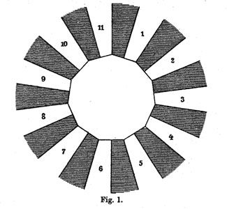
 The ramification data translates to the following statements about the Linienzuge : (a) it must be a tree ($\infty $ has one preimage), (b) there are exactly 11 (half)edges (the degree of the cover),