Last time I mentioned the talk “From noncommutative geometry to the tropical geometry of the scaling site” by Alain Connes, culminating in the canonical isomorphism (last slide of the talk)
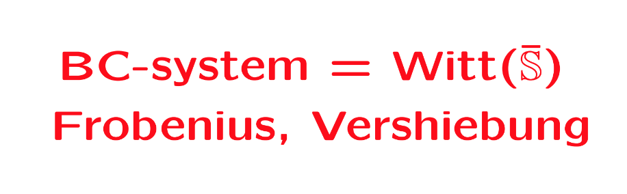
Or rather, what is actually proved in his paper with Caterina Consani BC-system, absolute cyclotomy and the quantized calculus (and which they conjectured previously to be the case in Segal’s Gamma rings and universal arithmetic), is a canonical isomorphism between the $\lambda$-rings
\[
\mathbb{Z}[\mathbb{Q}/\mathbb{Z}] \simeq \mathbb{W}_0(\overline{\mathbb{S}}) \]
The left hand side is the integral groupring of the additive quotient-group $\mathbb{Q}/\mathbb{Z}$, or if you prefer, $\mathbb{Z}[\mathbf{\mu}_{\infty}]$ the integral groupring of the multiplicative group of all roots of unity $\mathbf{\mu}_{\infty}$.
The power maps on $\mathbf{\mu}_{\infty}$ equip $\mathbb{Z}[\mathbf{\mu}_{\infty}]$ with a $\lambda$-ring structure, that is, a family of commuting endomorphisms $\sigma_n$ with $\sigma_n(\zeta) = \zeta^n$ for all $\zeta \in \mathbf{\mu}_{\infty}$, and a family of linear maps $\rho_n$ induced by requiring for all $\zeta \in \mathbf{\mu}_{\infty}$ that
\[
\rho_n(\zeta) = \sum_{\mu^n=\zeta} \mu \]
The maps $\sigma_n$ and $\rho_n$ are used to construct an integral version of the Bost-Connes algebra describing the Bost-Connes sytem, a quantum statistical dynamical system.
On the right hand side, $\mathbb{S}$ is the sphere spectrum (an object from stable homotopy theory) and $\overline{\mathbb{S}}$ its ‘algebraic closure’, that is, adding all abstract roots of unity.
The ring $\mathbb{W}_0(\overline{\mathbb{S}})$ is a generalisation to the world of spectra of the Almkvist-ring $\mathbb{W}_0(R)$ defined for any commutative ring $R$, constructed from pairs $(E,f)$ where $E$ is a projective $R$-module of finite rank and $f$ an $R$-endomorphism on it. Addition and multiplication are coming from direct sums and tensor products of such pairs, with zero element the pair $(0,0)$ and unit element the pair $(R,1_R)$. The ring $\mathbb{W}_0(R)$ is then the quotient-ring obtained by dividing out the ideal consisting of all zero-pairs $(E,0)$.
The ring $\mathbb{W}_0(R)$ becomes a $\lambda$-ring via the Frobenius endomorphisms $F_n$ sending a pair $(E,f)$ to the pair $(E,f^n)$, and we also have a collection of linear maps on $\mathbb{W}_0(R)$, the ‘Verschiebung’-maps which send a pair $(E,f)$ to the pair $(E^{\oplus n},F)$ with
\[
F = \begin{bmatrix} 0 & 0 & 0 & \cdots & f \\
1 & 0 & 0 & \cdots & 0 \\
0 & 1 & 0 & \cdots & 0 \\
\vdots & \vdots & \vdots & & \vdots \\
0 & 0 & 0 & \cdots & 1 \end{bmatrix} \]
Connes and Consani define a notion of modules and their endomorphisms for $\mathbb{S}$ and $\overline{\mathbb{S}}$, allowing them to define in a similar way the rings $\mathbb{W}_0(\mathbb{S})$ and $\mathbb{W}_0(\overline{\mathbb{S}})$, with corresponding maps $F_n$ and $V_n$. They then establish an isomorphism with $\mathbb{Z}[\mathbb{Q}/\mathbb{Z}]$ such that the maps $(F_n,V_n)$ correspond to $(\sigma_n,\rho_n)$.
But, do we really have the go to spectra to achieve this?
All this reminds me of an old idea of Yuri Manin mentioned in the introduction of his paper Cyclotomy and analytic geometry over $\mathbb{F}_1$, and later elaborated in section two of his paper with Matilde Marcolli Homotopy types and geometries below $\mathbf{Spec}(\mathbb{Z})$.
Take a manifold $M$ with a diffeomorphism $f$ and consider the corresponding discrete dynamical system by iterating the diffeomorphism. In such situations it is important to investigate the periodic orbits, or the fix-points $Fix(M,f^n)$ for all $n$. If we are in a situation that the number of fixed points is finite we can package these numbers in the Artin-Mazur zeta function
\[
\zeta_{AM}(M,f) = exp(\sum_{n=1}^{\infty} \frac{\# Fix(M,f^n)}{n}t^n) \]
and investigate the properties of this function.
To connect this type of problem to Almkvist-like rings, Manin considers the Morse-Smale dynamical systems, a structural stable diffeomorphism $f$, having a finite number of non-wandering points on a compact manifold $M$.
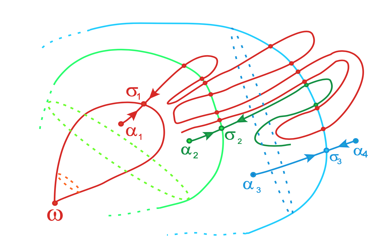
From Topological classification of Morse-Smale diffeomorphisms on 3-manifolds
In such a situation $f_{\ast}$ acts on homology $H_k(M,\mathbb{Z})$, which are free $\mathbb{Z}$-modules of finite rank, as a matrix $M_f$ having only roots of unity as its eigenvalues.
Manin argues that this action is similar to the action of the Frobenius on etale cohomology groups, in which case the eigenvalues are Weil numbers. That is, one might view roots of unity as Weil numbers in characteristic one.
Clearly, all relevant data $(H_k(M,\mathbb{Z}),f_{\ast})$ belongs to the $\lambda$-subring of $\mathbb{W}_0(\mathbb{Z})$ generated by all pairs $(E,f)$ such that $M_f$ is diagonalisable and all its eigenvalues are either $0$ or roots of unity.
If we denote for any ring $R$ by $\mathbb{W}_1(R)$ this $\lambda$-subring of $\mathbb{W}_0(R)$, probably one would obtain canonical isomorphisms
– between $\mathbb{W}_1(\mathbb{Z})$ and the invariant part of the integral groupring $\mathbb{Z}[\mathbb{Q}/\mathbb{Z}]$ for the action of the group $Aut(\mathbb{Q}/\mathbb{Z}) = \widehat{\mathbb{Z}}^*$, and
– between $\mathbb{Z}[\mathbb{Q}/\mathbb{Z}]$ and $\mathbb{W}_1(\mathbb{Z}(\mathbf{\mu}_{\infty}))$ where $\mathbb{Z}(\mathbf{\mu}_{\infty})$ is the ring obtained by adjoining to $\mathbb{Z}$ all roots of unity.