Category: math

Grothendieck meets Lacan

Published April 21, 2022 by lievenlb

Next month, a weekend-meeting is organised in Paris on Lacan et Grothendieck, l’impossible rencontre?.

Photo from Remembering my father, Jacques Lacan

Jacques Lacan was a French psychoanalyst and psychiatrist who has been called “the most controversial psycho-analyst since Freud”.

What’s the connection between Lacan and Grothendieck? Here’s Stephane Dugowson‘s take (G-translated):

“As we know, Lacan was passionate about certain mathematics, notably temporal logic and the theory of knots, where he thought he found material for advancing the theory of psychoanalysis. For his part, Grothendieck testifies in his non-strictly mathematical writings to his passion for the psyche, as shown by many pages of his Récoltes et Semailles just published by Gallimard (in January 2022), or even, among the tens of thousands of pages discovered at his death and of which we know almost nothing, the 3700 pages of mathematics grouped under the title ‘Structure of the Psyche’.

One might therefore be surprised that the two geniuses never met. In fact, a lunch did take place in the early 1970s organized by the mathematician and psychoanalyst Daniel Sibony. But a lunch does not necessarily make a meeting, and it seems that this one unfortunately did not happen.”

As it is ‘bon ton’ these days in Parisian circles to utter the word ‘topos’, several titles of the talks given at the meeting contain that word.

There’s Stephane Dugowson‘s talk on “Logique du topos borroméen et autres logiques à trois points”.

Lacan used the Borromean link to illustrate his concepts of the Real, Symbolic, and Imaginary (RSI). For more on this, please read chapter 6 of Lionel Baily’s excellent introduction to Lacan’s work Lacan, A Beginner’s Guide.

The Borromean topos is an example of Dugowson’s toposes associated to his ‘connectivity spaces’. From his paper Définition du topos d’un espace connectif I gather that the objects in the Borromean topos consist of a triple of set-maps from a set $A$ (the global sections) to sets $A_x,A_y$ and $A_z$ (the restrictions to three disconnected ‘opens’).

\[
\xymatrix{& A \ar[rd] \ar[d] \ar[ld] & \\ A_x & A_y & A_z} \]

This seems to be a topos with a Boolean logic, but perhaps there are other 3-point connectivity spaces with a non-Boolean Heyting subobject classifier.

There’s Daniel Sibony‘s talk on “Mathématiques et inconscient”. Sibony is a French mathematician, turned philosopher and psychoanalyst, l’inconscient is an important concept in Lacan’s work.

Here’s a nice conversation between Daniel Sibony and Alain Connes on the notions of ‘time’ and ‘truth’.

In the second part (starting around 57.30) Connes brings up toposes whose underlying logic is much subtler than brute ‘true’ or ‘false’ statements. He discusses the presheaf topos on the additive monoid $\mathbb{N}_+$ which leads to statements which are ‘one step from the truth’, ‘two steps from the truth’ and so on. It is also the example Connes used in his talk Un topo sur les topos.

Alain Connes himself will also give a talk at the meeting, together with Patrick Gauthier-Lafaye, on “Un topos sur l’inconscient”.

It appears that Connes and Gauthier-Lafaye have written a book on the subject, A l’ombre de Grothendieck et de Lacan : un topos sur l’inconscient. Here’s the summary (G-translated):

“The authors present the relevance of the mathematical concept of topos, introduced by A. Grothendieck at the end of the 1950s, in the exploration of the structure of the unconscious.”

The book will be released on May 11th.

2 Comments

Mamuth to Elephant (3)

Published March 13, 2022 by lievenlb

Until now, we’ve looked at actions of groups (such as the $T/I$ or $PLR$-group) or (transformation) monoids (such as Noll’s monoid) on special sets of musical elements, in particular the twelve pitch classes $\mathbb{Z}_{12}$, or the set of all $24$ major and minor chords.

Elephant-lovers recognise such settings as objects in the presheaf topos on the one-object category $\mathbf{M}$ corresponding to the group or monoid. That is, we look at contravariant functors $\mathbf{M} \rightarrow \mathbf{Sets}$.

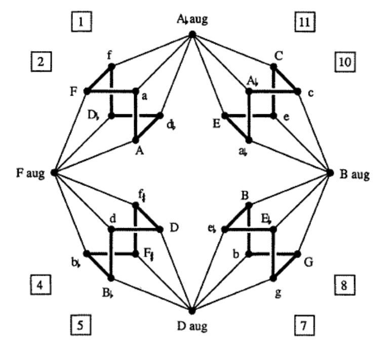
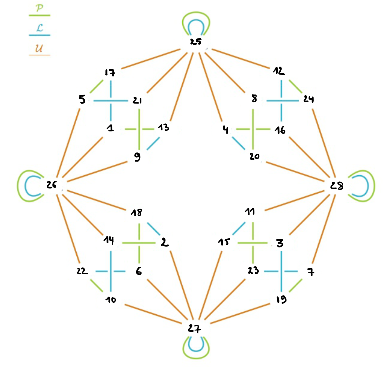
Last time we’ve encountered the ‘Cube Dance Grap’ which depicts a particular relation among the major, minor, and augmented chords.

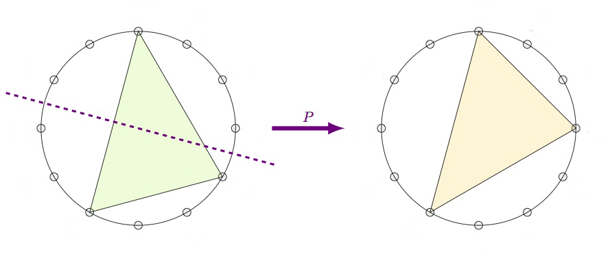
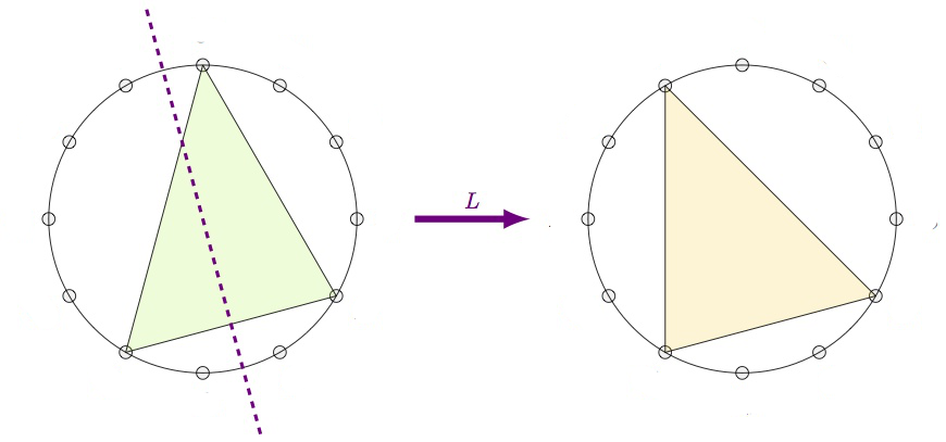
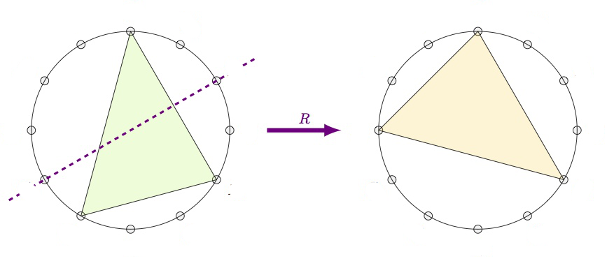
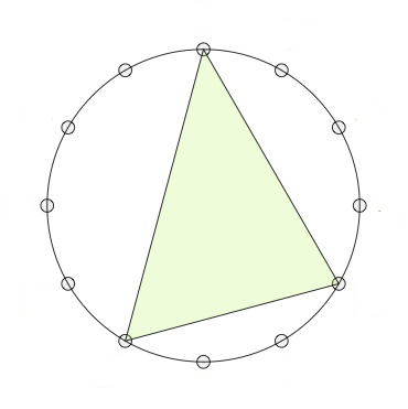
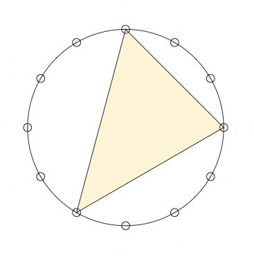
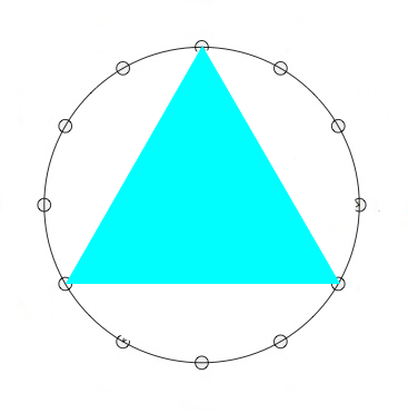
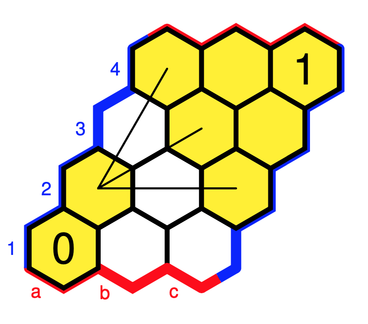
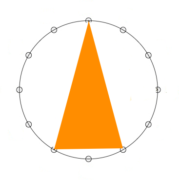
Recall that the twelve major chords (numbered for $1$ to $12$) are the ordered triples of tones in $\mathbb{Z}_{12}$ of the form $(n,n+4,n+7)$ (such as the triangle on the left). The twelve minor chords (numbered from $13$ to $24$) are the ordered triples $(n,n+3,n+7)$ (such as the middle triangle). The four augmented chords (numbered from $25$ to $28$) are the triples of the form $(n,n+4,n+8)$ (such as the rightmost triangle).

The Cube Dance Graph relates two of these chords when they share two tones (pitch classes) whereas the remaining tones differ by a halftone.

Picture modified from this post.

We can separate this symmetric binary relation into three sub-relations: the extension of the $P$ and $L$-operations on major and minor chords to the augmented ones (these are transformations), and the remaining relation $U$ which connects the major and minor chords to the augmented chords (and which is not a transformation).

Binary relations on the same set can be composed, so we get a monoid $\mathbf{M}$ generated by the three relations $P,L$ and $U$. The action of $\mathbf{M}$ on the $28$ chords no longer gives us an ordinary presheaf (because $U$ is not a transformation), but a relational presheaf as in the paper On the use of relational presheaves in transformational music theory by Alexandre Popoff.

That is, the action defines a contravariant functor $\mathbf{M} \rightarrow \mathbf{Rel}$ where $\mathbf{Rel}$ is the category (actually a $2$-category) of sets, but with binary relations as morphisms (that is, $Hom(X,Y)$ is all subsets of $X \times Y$), and the natural notion of composition of such relations. The $2$-morphism between relations is that of inclusion.

To compute with monoids generated by binary relations in GAP one needs to download, compile and load the package semigroups, and to represent the binary relations as partitioned binary relations as in the paper by Martin and Mazorchuk.

This is a bit more complicated than working with ordinary transformations:

But then, GAP quickly tells us that $\mathbf{M}$ is a monoid consisting of $40$ elements.

gap> M:=Semigroup([P,L,U]); gap> Size(M); 40

The Semigroups-package can also compute Green’s relations and tells us that there are seven such $R$-classes, four consisting of $6$ elements, two of four, and one of eight elements. These are also visible in the Cayley graph, exactly as last time.

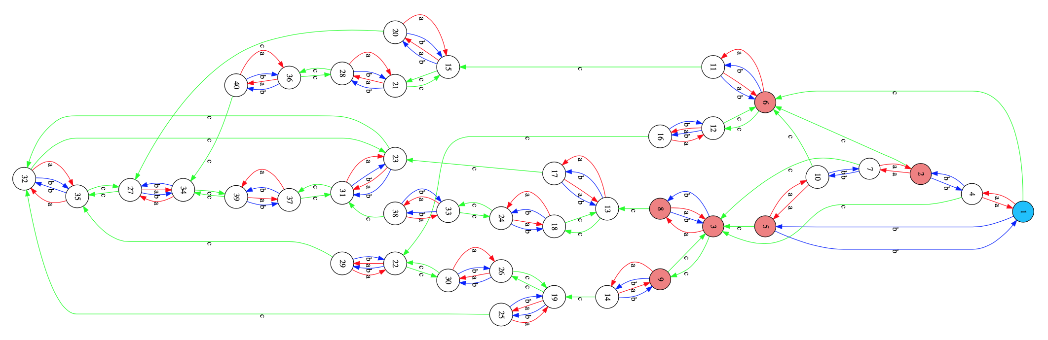
Or, if you prefer the cleaner picture of the Cayley graph from the paper Relational poly-Klumpenhouwer networks for transformational and voice-leading analysis by Popoff, Andreatta and Ehresmann.

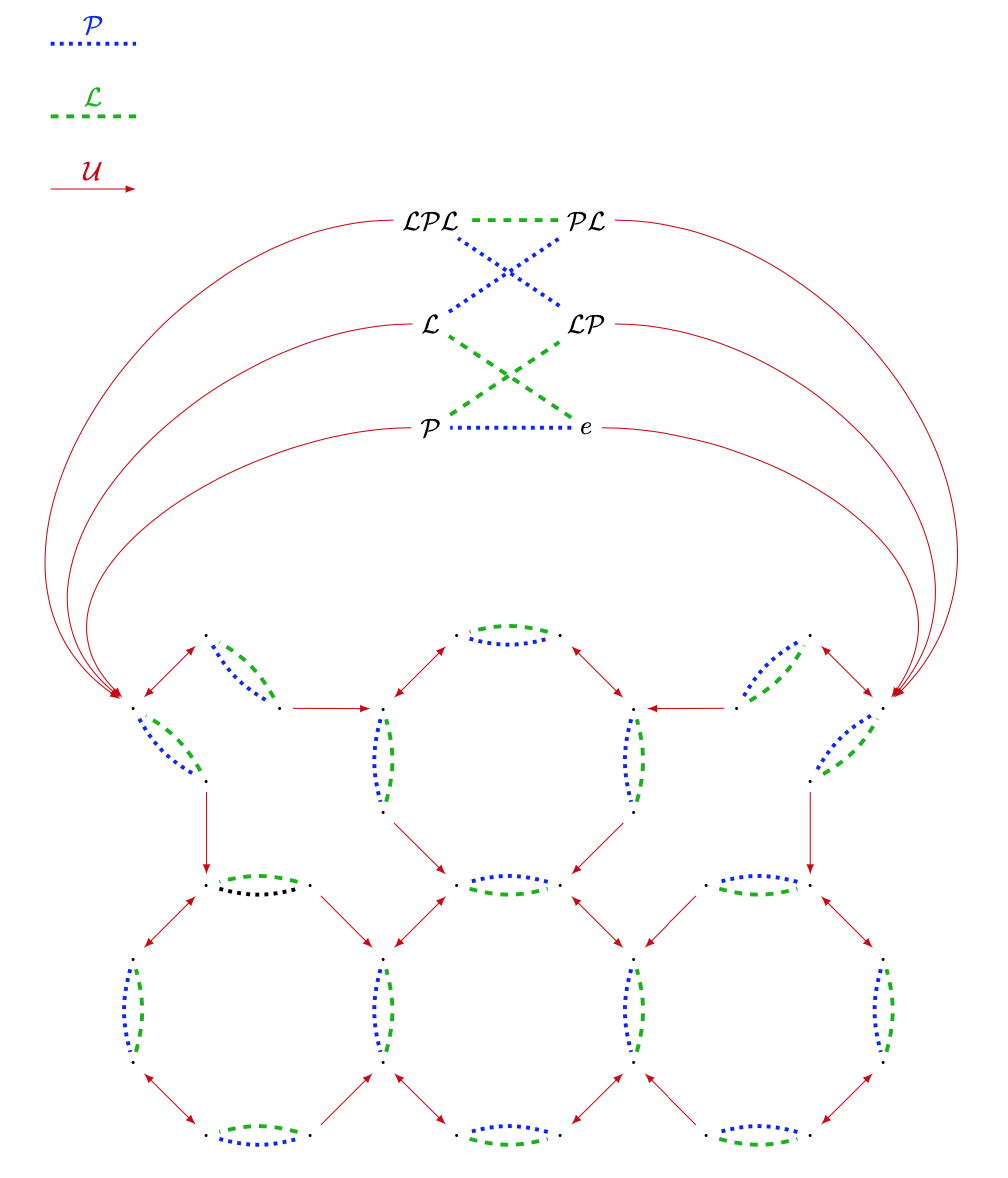
This then allows us to compute the Heyting algebra of the subobject classifier, and all the Grothendieck topologies, at least for the ordinary presheaf topos of $\mathbf{M}$-sets, not for the relational presheaves we need here.

We can consider the same binary relation on the larger set of triads when we add the suspended triads. These are the ordered triples in $\mathbb{Z}_{12}$ of the form $(n,n+5,n+7)$, as in the rightmost triangle below.

There are twelve suspended chords (numbered from $29$ to $40$), so we now have a binary relation $T$ on a set of $40$ triads.

The relation $T$ is too coarse, and the art is to subdivide $T$ is disjoint sub-relations which are musically significant, between major and minor triads, between major/minor and augmented triads, and so on.

For each such partition we can then consider the monoids generated by these sub-relations.

In his paper, Popoff suggest relevant sub-relations $P,L,T_U,T_V$ and $T_U \cup T_V$ of $T$ which in our numbering of the $40$ chords can be represented by these PBR’s (assuming I made no mistakes…ADDED march 24th: I did make a mistake in the definition of L, see comment by Alexandre Popoff, below the corect L):

P:=PBR([[-13],[-14],[-15],[-16],[-17],[-18],[-19],[-20],[-21],[-22],[-23],[-24],[-1],[-2],[-3],[-4],[-5],[-6],[-7],[-8],[-9],[-10],[-11],[-12],[-25],[-26],[-27],[-28],[-36],[-37],[-38],[-39],[-40],[-29],[-30],[-31],[-32],[-33],[-34],[-35]],[[13],[14],[15],[16],[17],[18],[19],[20],[21],[22],[23],[24],[1],[2],[3],[4],[5],[6],[7],[8],[9],[10],[11],[12],[25],[26],[27],[28],[34],[35],[36],[37],[38],[39],[40],[29],[30],[31],[32],[33]]); L:=PBR([[-17],[-18],[-19],[-20],[-21],[-22],[-23],[-24],[-13],[-14],[-15],[-16],[-9],[ -10],[-11],[-12],[-1],[-2],[-3],[-4],[-5],[-6],[-7],[-8],[-25],[-26],[-27],[-28],[-29], [-30],[-31],[-32],[-33],[-34],[-35],[-36],[-37],[-38],[-39],[-40]],[[17], [18], [19], [ 20],[21],[22],[23],[24],[13],[14],[15],[16],[9],[10],[11],[12],[1],[2],[3],[4],[5], [6], [7],[8],[25],[26],[27],[28],[29],[30],[31],[32],[33],[34],[35],[36],[37],[38],[39],[40] ]); TU:=PBR([[-26],[-27],[-28],[-25],[-26],[-27],[-28],[-25],[-26],[-27],[-28],[-25],[-25],[-26],[-27],[-28],[-25],[-26],[-27],[-28],[-25],[-26],[-27],[-28],[-4,-8,-12,-13,-17,-21],[-1,-5,-9,-14,-18,-22],[-2,-6,-10,-15,-19,-23],[-3,-7,-11,-16,-20,-24],[],[],[],[],[],[],[],[],[],[],[],[]],[[26],[27],[28],[25],[26],[27],[28],[25],[26],[27],[28],[25],[25],[26],[27],[28],[25],[26],[27],[28],[25],[26],[27],[28],[4,8,12,13,17,21],[1,5,9,14,18,22],[2,6,10,15,19,23],[3,7,11,16,20,24],[],[],[],[],[],[],[],[],[],[],[],[]]); TV:=PBR([[-29],[-30],[-31],[-32],[-33],[-34],[-35],[-36],[-37],[-38],[-39],[-40],[-36],[-37],[-38],[-39],[-40],[-29],[-30],[-31],[-32],[-33],[-34],[-35],[],[],[],[],[-1,-18],[-2,-19],[-3,-20],[-4,-21],[-5,-22],[-6,-23],[-7,-24],[-8,-13],[-9,-14],[-10,-15],[-11,-16],[-12,-17]],[[29],[30],[31],[32],[33],[34],[35],[36],[37],[38],[39],[40],[36],[37],[38],[39],[40],[29],[30],[31],[32],[33],[34],[35],[],[],[],[],[1,18],[2,19],[3,20],[4,21],[5,22],[6,23],[7,24],[8,13],[9,14],[10,15],[11,16],[12,17]]); TUV:=PBR([[-26,-29],[-27,-30],[-28,-31],[-25,-32],[-26,-33],[-27,-34],[-28,-35],[-25,-36],[-26,-37],[-27,-38],[-28,-39],[-25,-40],[-25,-36],[-26,-37],[-27,-38],[-28,-39],[-25,-40],[-26,-29],[-27,-30],[-28,-31],[-25,-32],[-26,-33],[-27,-34],[-28,-35],[-4,-8,-12,-13,-17,-21],[-1,-5,-9,-14,-18,-22],[-2,-6,-10,-15,-19,-23],[-3,-7,-11,-16,-20,-24],[-1,-18],[-2,-19],[-3,-20],[-4,-21],[-5,-22],[-6,-23],[-7,-24],[-8,-13],[-9,-14],[-10,-15],[-11,-16],[-12,-17]],[[26,29],[27,30],[28,31],[25,32],[26,33],[27,34],[28,35],[25,36],[26,37],[27,38],[28,39],[25,40],[25,36],[26,37],[27,38],[28,39],[25,40],[26,29],[27,30],[28,31],[25,32],[26,33],[27,34],[28,35],[4,8,12,13,17,21],[1,5,9,14,18,22],[2,6,10,15,19,23],[3,7,11,16,20,24],[1,18],[2,19],[3,20],[4,21],[5,22],[6,23],[7,24],[8,13],[9,14],[10,15],[11,16],[12,17]]);

The resulting monoids are huge:

gap> G:=Semigroup([P,L,TU,TV]); gap> Size(G); 473293 gap> H:=Semigroup([P,L,TUV]); gap> Size(H); 994624

~~In Popoff’s paper these monoids have sizes respectively $473,293$ and $994,624$. Strangely, the offset is in both cases $144=12^2$.~~ (Added march 24: with the correct L I get the same sizes as in Popoff’s paper).

Perhaps we should try to transform such relational presheaves to ordinary presheaves.

One approach is to use the Grothendieck construction and associate to a set with such a relational monoid action a directed graph, coloured by the elements of the monoid. That is, an object in the presheaf topos of the category
\[
\xymatrix{C & E \ar[l]^c \ar@/^2ex/[r]^s \ar@/_2ex/[r]_t & V} \]
and then we should consider the slice topos over the one-vertex bouquet graph with one loop for each element in the monoid.

If you want to have more details on the musical side of things, for example if you want to know what the opening twelve chords of “Take a Bow” by Muse have to do with the Cube Dance graph, here are some more papers:

A categorical generalization of Klumpenhouwer networks, A. Popoff, M. Andreatta and A. Ehresmann.

From K-nets to PK-nets: a categorical approach, A. Popoff, M. Andreatta and A. Ehresmann.

From a Categorical Point of View: K-Nets as Limit Denotators, G. Mazzola and M. Andreatta.

6 Comments

Mamuth to Elephant (2)

Published March 8, 2022 by lievenlb

Last time, we’ve viewed major and minor triads (chords) as inscribed triangles in a regular $12$-gon.

If we move clockwise along the $12$-gon, starting from the endpoint of the longest edge (the root of the chord, here the $0$-vertex) the edges skip $3,2$ and $4$ vertices (for a major chord, here on the left the major $0$-chord) or $2,3$ and $4$ vertices (for a minor chord, here on the right the minor $0$-chord).

The symmetries of the $12$-gon, the dihedral group $D_{12}$, act on the $24$ major- and minor-chords transitively, preserving the type for rotations, and interchanging majors with minors for reflections.

Mathematical Music Theoreticians (MaMuTh-ers for short) call this the $T/I$-group, and view the rotations of the $12$-gon as transpositions $T_k : x \mapsto x+k~\text{mod}~12$, and the reflections as involutions $I_k : x \mapsto -x+k~\text{mod}~12$.

Note that the elements of the $T/I$-group act on the vertices of the $12$-gon, from which the action on the chord-triangles follows.

There is another action on the $24$ major and minor chords, mapping a chord-triangle to its image under a reflection in one of its three sides.

Note that in this case the reflection $I_k$ used will depend on the root of the chord, so this action on the chords does not come from an action on the vertices of the $12$-gon.

There are three such operations: (pictures are taken from Alexandre Popoff’s blog, with the ‘funny names’ removed)

The $P$-operation is reflection in the longest side of the chord-triangle. As the longest side is preserved, $P$ interchanges the major and minor chord with the same root.

The $L$-operation is refection in the shortest side. This operation interchanges a major $k$-chord with a minor $k+4~\text{mod}~12$-chord.

Finally, the $R$-operation is reflection in the middle side. This operation interchanges a major $k$-chord with a minor $k+9~\text{mod}~12$-chord.

From this it is already clear that the group generated by $P$, $L$ and $R$ acts transitively on the $24$ major and minor chords, but what is this $PLR$-group?

If we label the major chords by their root-vertex $1,2,\dots,12$ (GAP doesn’t like zeroes), and the corresponding minor chords $13,14,\dots,24$, then these operations give these permutations on the $24$ chords:

P:=(1,13)(2,14)(3,15)(4,16)(5,17)(6,18)(7,19)(8,20)(9,21)(10,22)(11,23)(12,24) L:=(1,17)(2,18)(3,19)(4,20)(5,21)(6,22)(7,23)(8,24)(9,13)(10,14)(11,15)(12,16) R:=(1,22)(2,23)(3,24)(4,13)(5,14)(6,15)(7,16)(8,17)(9,18)(10,19)(11,20)(12,21)

Then GAP gives us that the $PLR$-group is again isomorphic to $D_{12}$:

gap> G:=Group(P,L,R);; gap> Size(G); 24 gap> IsDihedralGroup(G); true

In fact, if we view both the $T/I$-group and the $PLR$-group as subgroups of the symmetric group $Sym(24)$ via their actions on the $24$ major and minor chords, these groups are each other centralizers! That is, the $T/I$-group and $PLR$-group are dual to each other.

For more on this, there’s a beautiful paper by Alissa Crans, Thomas Fiore and Ramon Satyendra: Musical Actions of Dihedral Groups.

What does this new MaMuTh info learns us more about our Elephant, the Topos of Triads, studied by Thomas Noll?

Last time we’ve seen the eight element triadic monoid $T$ of all affine maps preserving the three tones $\{ 0,4,7 \}$ of the major $0$-chord, computed the subobject classified $\Omega$ of the corresponding topos of presheaves, and determined all its six Grothendieck topologies, among which were these three:

Why did we label these Grothendieck topologies (and corresponding elements of $\Omega$) by $P$, $L$ and $R$?

We’ve seen that the sheafification of the presheaf $\{ 0,4,7 \}$ in the triadic topos under the Grothendieck topology $j_P$ gave us the sheaf $\{ 0,3,4,7 \}$, and these are the tones of the major $0$-chord together with those of the minor $0$-chord, that is the two chords in the $\langle P \rangle$-orbit of the major $0$-chord. The group $\langle P \rangle$ is the cyclic group $C_2$.

For the sheafication with respect to $j_L$ we found the $T$-set $\{ 0,3,4,7,8,11 \}$ which are the tones of the major and minor $0$-,$4$-, and $8$-chords. Again, these are exactly the six chords in the $\langle P,L \rangle$-orbit of the major $0$-chord. The group $\langle P,L \rangle$ is isomorphic to $Sym(3)$.

The $j_R$-topology gave us the $T$-set $\{ 0,1,3,4,6,7,9,10 \}$ which are the tones of the major and minor $0$-,$3$-, $6$-, and $9$-chords, and lo and behold, these are the eight chords in the $\langle P,R \rangle$-orbit of the major $0$-chord. The group $\langle P,R \rangle$ is the dihedral group $D_4$.

More on this can be found in the paper Commuting Groups and the Topos of Triads by Thomas Fiore and Thomas Noll.

The operations $P$, $L$ and $R$ on major and minor chords are reflexions in one side of the chord-triangle, so they preserve two of the three tones. There’s a distinction between the $P$ and $L$ operations and $R$ when it comes to how the third tone changes.

Under $P$ and $L$ the third tone changes by one halftone (because the corresponding sides skip an even number of vertices), whereas under $R$ the third tone changes by two halftones (a full tone), see the pictures above.

The $\langle P,L \rangle = Sym(3)$ subgroup divides the $24$ chords in four orbits of six chords each, three major chords and their corresponding minor chords. These orbits consist of the

$0$-, $4$-, and $8$-chords (see before)
$1$-, $5$-, and $9$-chords
$2$-, $6$-, and $10$-chords
$3$-, $7$-, and $11$-chords

and we can view each of these orbits as a cycle tracing six of the eight vertices of a cube with one pair of antipodal points removed.

These four ‘almost’ cubes are the NE-, SE-, SW-, and NW-regions of the Cube Dance Graph, from the paper Parsimonious Graphs by Jack Douthett and Peter Steinbach.

To translate the funny names to our numbers, use this dictionary (major chords are given by a capital letter):

The four extra chords (at the N, E, S, and P places) are augmented triads. They correspond to the triads $(0,4,8),~(1,5,9),~(2,6,10)$ and $(3,7,11)$.

That is, two triads are connected by an edge in the Cube Dance graph if they share two tones and differ by an halftone in the third tone.

This graph screams for a group or monoid acting on it. Some of the edges we’ve already identified as the action of $P$ and $L$ on the $24$ major and minor triads. Because the triangle of an augmented triad is equilateral, we see that they are preserved under $P$ and $L$.

But what about the edges connecting the regular triads to the augmented ones? If we view each edge as two directed arrows assigned to the same operation, we cannot do this with a transformation because the operation sends each augmented triad to six regular triads.

Alexandre Popoff, Moreno Andreatta and Andree Ehresmann suggest in their paper Relational poly-Klumpenhouwer networks for transformational and voice-leading analysis that one might use a monoid generated by relations, and they show that there is such a monoid with $40$ elements acting on the Cube Dance graph.

Popoff claims that usual presheaf toposes, that is contravariant functors to $\mathbf{Sets}$ are not enough to study transformational music theory. He suggest to use instead functors to $\mathbf{Rel}$, that is Sets with as the morphisms binary relations, and their compositions.

Another Elephant enters the room…

(to be continued)