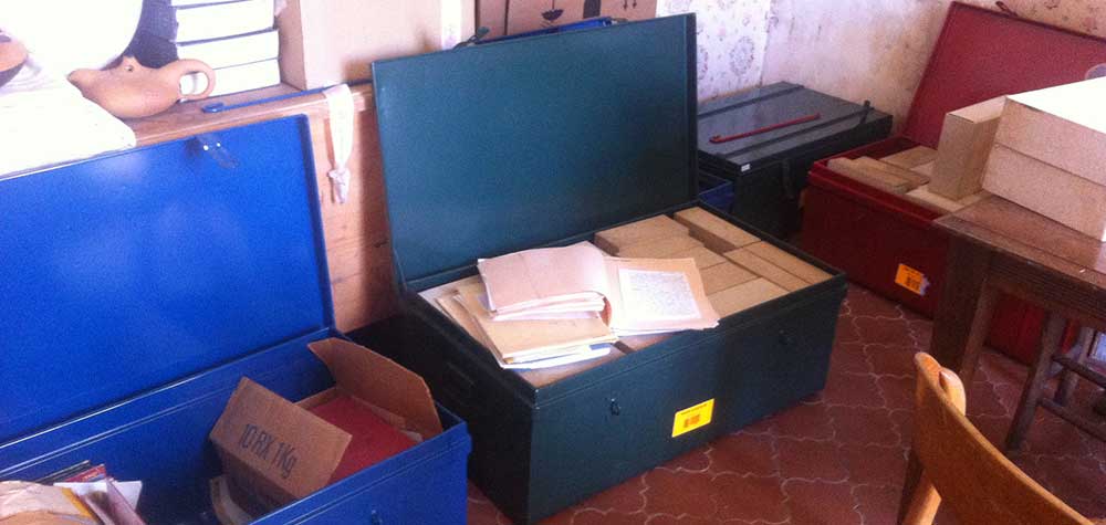
I’m retiring in two weeks so I’m cleaning out my office.
So far, I got rid of almost all paper-work and have split my book-collection in two: the books I want to take with me, and those anyone can grab away.
Here’s the second batch (math/computer books in the middle, popular science to the right, thrillers to the left).
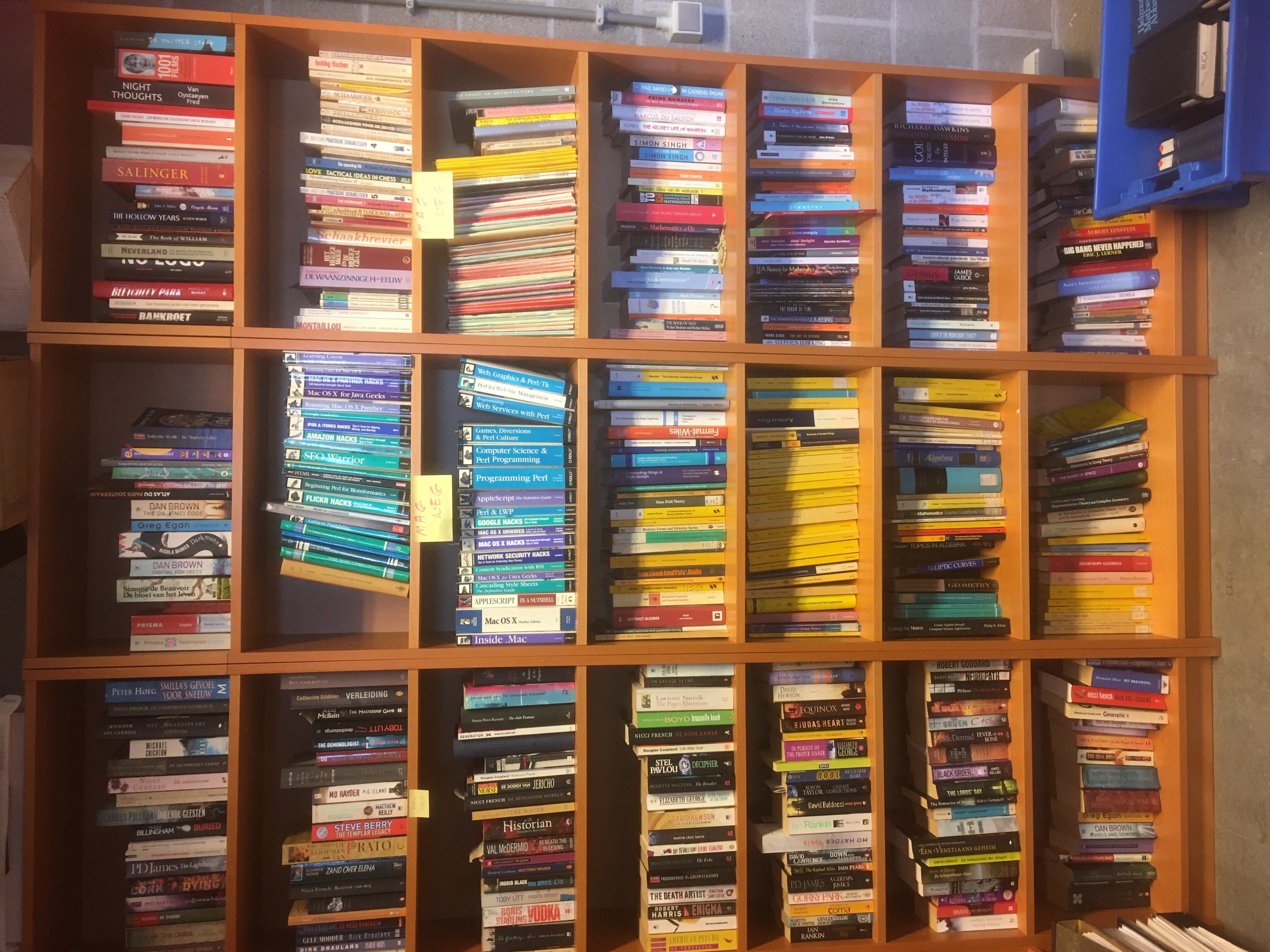
If you’re interested in some of these books (click for a larger image, if you want to zoom in) and are willing to pay the postage, leave a comment and I’ll try to send them if they survive the current ‘take-away’ phase.
Here are two books I definitely want to keep. On the left, an original mimeographed version of Mumford’s ‘Red Book’.
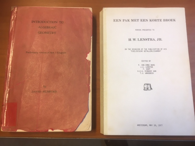
On the right, ‘Een pak met een korte broek’ (‘A suit with shorts’), a collection of papers by family and friends, presented to Hendrik Lenstra on the occasion of the defence of his Ph.D. thesis on Euclidean number-fields, May 18th 1977.
If the title intrigues you, a photo of young Hendrik in suit and shorts is included.
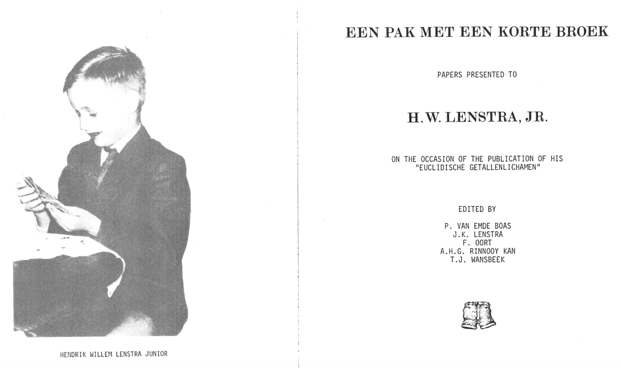
This collection includes hilarious ‘papers’ by famous people including
- ‘A headache-causing problem’ by Conway (J.H.), Paterson (M.S.), and Moscow (U.S.S.R.)
- ‘A projective plain of order ten’ by A.M. Odlyzko and N.J.A. Sloane
- ‘La chasse aux anneaux principaux non-Euclidiens dans l’enseignement’ by Pierre Samuel
- ‘On time-like theorems’ by Michiel Hazewinkel
- ‘She loves me, she loves me not’ by Richard K. Guy
- ‘Theta invariants for affine root systems’ by E.J.N. Looijenga
- ‘The prime of primes’ by F. Lenstra and A.J. Oort
- (and many more, most of them in Dutch)
Perhaps I can do a couple of posts on some of these papers. It might break this clean-up routine.
One Comment