Category: geometry

the topos of unconsciousness

Published May 14, 2022 by lievenlb

Since wednesday, as mentioned last time, the book by Alain Connes and Patrick Gauthier-Lafaye: “A l’ombre de Grothendieck et de Lacan, un topos sur l’inconscient” is available in the better bookshops.

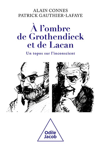
There’s no need to introduce Alain Connes on this blog. Patrick Gauthier-Lafaye is a French psychiatrist and psycho-analyst, working in Strassbourg.

The book is a lengthy dialogue in which the authors try to find a use for topos theory in Jaques Lacan’s psycho-analytical view of the unconscious.

If you are a complete Lacanian virgin, it may be helpful to browse through “Lacan, a beginners guide” (by Lionel Bailly) first.

If this left you bewildered, for example by Lacan’s strange (ab)use of mathematics, rest assured, you’re not alone.

It is no coincidence that Lacan’s works are the first case-study in the book “Fashionable Nonsense: Postmodern Intellectuals’ Abuse of Science” by Alan Sokal (the one of the hoax) and Jean Bricmont. You can download the book from this link.

If now you feel that Sokal and Bricmont are way too harsh on Lacan, I urge you to have a go at the book “Writing the structures of the subject, Lacan and topology” by Will Greenshields.

If you don’t have the time or energy for this, let me give you one illustrative example: the topological explanation of Lacan’s formula of fantasy:

\[
\$~\diamond~a \]

Loosely speaking this formula says “the barred subject stands within a circular relationship to the objet petit a (the object of desire), one part of which is determined by alienation, the other by separation”.

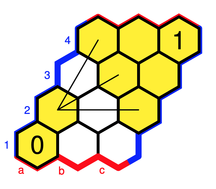
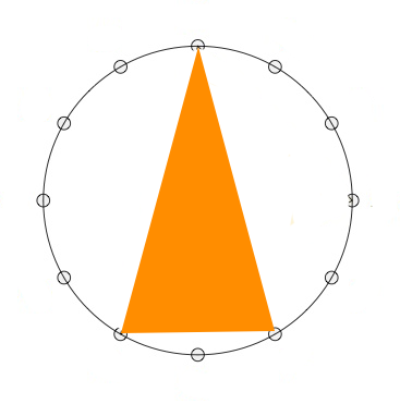
Lacan was obsessed with the immersion of the projective plane $\mathbb{P}^2(\mathbb{R})$ into $\mathbb{R}^3$ as the cross-cap. Here’s an image of it from his 1966-67 seminar on ‘Logique du fantasme’ (213 pages).

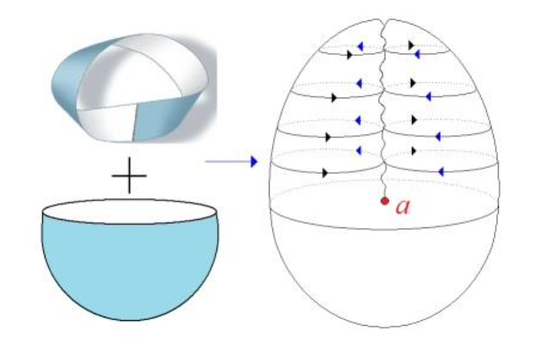
This image includes the position of the objet petit $a$ as the end point of the self-intersection curve, which itself is referred to as the ‘castration’, or the ‘phallus’, or whatever.

Brace yourself for the ‘explanation’ of $\$~\diamond~a$: if you walk twice around $a$ this divides the cross-cap into a disk and a Mobius-strip!

The mathematics is correct but I fail to see how this helps the psycho-analyst in her therapy. But hey, everyone will tell you I have absolutely no therapeutic talent.

Let’s return to the brand new book by Alain Connes and Patrick Gauthier-Lafaye: “A l’ombre de Grothendieck et de Lacan, un topos sur l’inconscient”.

It was to be expected that they would defend Lacan’s exploitation of (surface) topology by saying that he was just unfortunate not to have the more general notion of toposes available, as well as their much subtler logic. Perhaps someone should write a fictional parody on Greenshields book: “Lacan and the topos”…

Connes’ first attempt to construct the topos of unconsciousness was also not much of a surprise. According to Lacan the unconscious is ‘structured like a language’.

So, a natural approach might be to start with a ‘dictionary’-category (words and relations between them) or any other known use of a category in linguistics. A good starting point to read up on this is the blog post A new application of category theory in linguistics.

Eventually they settled for a much more ambitious project. To Connes and Gauthier-Lafaye every individual has her own topos and corresponding logic.

They don’t specify how to construct these individual toposes, but postulate that they are all connected to a classifying topos, which is their incarnation of the world of ‘myths’ and ‘fantasies’.

Surely an idea Lacan would have liked. Underlying the unconscious must be, according to Connes and Gauthier-Lafaye, a geometric theory! That is, it can be fully described by first order sentences.

Lacan himself used already some first order sequences in his teachings, such as in his logic of sexuation:

\[
\forall x~(\Phi~x)~\quad \text{but also} \quad \exists x~\neg~(\Phi~x) \]

where $\Phi~x$ is the phallic function. Quoting from Greenshield’s book:

“While all (the sons) are subject to ($\forall x$) the law of castration ($\Phi~x$), we also learn that this law nevertheless resides upon an exception: there exists a subject ($\exists x$) that is not subject to this law ($\neg \Phi~x$). This exception is embodied by the despotic father who, not being subject to the phallic function, experiences an impossible mode of totalised jouissance (he enjoys all the women). He is, quite simply, the exception that proves the law a necessary beyond that enables the law’s geometric bounds to be defined.”

It will be quite hard (but probably great fun for psycho-analysts) to turn the whole of Lacanian theory on the unconscious into a coherent geometric theory, construct its classifying topos, and apply the Joyal-Reyes theorem to get at the individual cases/toposes.

I’m sure there are much deeper insights to be gained from Connes’ and Gauthier-Lafaye’s book, but this is what i got from a first, fast, cursory reading of it.

Grothendieck meets Lacan

Published April 21, 2022 by lievenlb

Next month, a weekend-meeting is organised in Paris on Lacan et Grothendieck, l’impossible rencontre?.

Photo from Remembering my father, Jacques Lacan

Jacques Lacan was a French psychoanalyst and psychiatrist who has been called “the most controversial psycho-analyst since Freud”.

What’s the connection between Lacan and Grothendieck? Here’s Stephane Dugowson‘s take (G-translated):

“As we know, Lacan was passionate about certain mathematics, notably temporal logic and the theory of knots, where he thought he found material for advancing the theory of psychoanalysis. For his part, Grothendieck testifies in his non-strictly mathematical writings to his passion for the psyche, as shown by many pages of his Récoltes et Semailles just published by Gallimard (in January 2022), or even, among the tens of thousands of pages discovered at his death and of which we know almost nothing, the 3700 pages of mathematics grouped under the title ‘Structure of the Psyche’.

One might therefore be surprised that the two geniuses never met. In fact, a lunch did take place in the early 1970s organized by the mathematician and psychoanalyst Daniel Sibony. But a lunch does not necessarily make a meeting, and it seems that this one unfortunately did not happen.”

As it is ‘bon ton’ these days in Parisian circles to utter the word ‘topos’, several titles of the talks given at the meeting contain that word.

There’s Stephane Dugowson‘s talk on “Logique du topos borroméen et autres logiques à trois points”.

Lacan used the Borromean link to illustrate his concepts of the Real, Symbolic, and Imaginary (RSI). For more on this, please read chapter 6 of Lionel Baily’s excellent introduction to Lacan’s work Lacan, A Beginner’s Guide.

The Borromean topos is an example of Dugowson’s toposes associated to his ‘connectivity spaces’. From his paper Définition du topos d’un espace connectif I gather that the objects in the Borromean topos consist of a triple of set-maps from a set $A$ (the global sections) to sets $A_x,A_y$ and $A_z$ (the restrictions to three disconnected ‘opens’).

\[
\xymatrix{& A \ar[rd] \ar[d] \ar[ld] & \\ A_x & A_y & A_z} \]

This seems to be a topos with a Boolean logic, but perhaps there are other 3-point connectivity spaces with a non-Boolean Heyting subobject classifier.

There’s Daniel Sibony‘s talk on “Mathématiques et inconscient”. Sibony is a French mathematician, turned philosopher and psychoanalyst, l’inconscient is an important concept in Lacan’s work.

Here’s a nice conversation between Daniel Sibony and Alain Connes on the notions of ‘time’ and ‘truth’.

In the second part (starting around 57.30) Connes brings up toposes whose underlying logic is much subtler than brute ‘true’ or ‘false’ statements. He discusses the presheaf topos on the additive monoid $\mathbb{N}_+$ which leads to statements which are ‘one step from the truth’, ‘two steps from the truth’ and so on. It is also the example Connes used in his talk Un topo sur les topos.

Alain Connes himself will also give a talk at the meeting, together with Patrick Gauthier-Lafaye, on “Un topos sur l’inconscient”.

It appears that Connes and Gauthier-Lafaye have written a book on the subject, A l’ombre de Grothendieck et de Lacan : un topos sur l’inconscient. Here’s the summary (G-translated):

“The authors present the relevance of the mathematical concept of topos, introduced by A. Grothendieck at the end of the 1950s, in the exploration of the structure of the unconscious.”

The book will be released on May 11th.

2 Comments

Mamuth to Elephant (3)

Published March 13, 2022 by lievenlb

Until now, we’ve looked at actions of groups (such as the $T/I$ or $PLR$-group) or (transformation) monoids (such as Noll’s monoid) on special sets of musical elements, in particular the twelve pitch classes $\mathbb{Z}_{12}$, or the set of all $24$ major and minor chords.

Elephant-lovers recognise such settings as objects in the presheaf topos on the one-object category $\mathbf{M}$ corresponding to the group or monoid. That is, we look at contravariant functors $\mathbf{M} \rightarrow \mathbf{Sets}$.

Last time we’ve encountered the ‘Cube Dance Grap’ which depicts a particular relation among the major, minor, and augmented chords.

Recall that the twelve major chords (numbered for $1$ to $12$) are the ordered triples of tones in $\mathbb{Z}_{12}$ of the form $(n,n+4,n+7)$ (such as the triangle on the left). The twelve minor chords (numbered from $13$ to $24$) are the ordered triples $(n,n+3,n+7)$ (such as the middle triangle). The four augmented chords (numbered from $25$ to $28$) are the triples of the form $(n,n+4,n+8)$ (such as the rightmost triangle).

The Cube Dance Graph relates two of these chords when they share two tones (pitch classes) whereas the remaining tones differ by a halftone.

Picture modified from this post.

We can separate this symmetric binary relation into three sub-relations: the extension of the $P$ and $L$-operations on major and minor chords to the augmented ones (these are transformations), and the remaining relation $U$ which connects the major and minor chords to the augmented chords (and which is not a transformation).

Binary relations on the same set can be composed, so we get a monoid $\mathbf{M}$ generated by the three relations $P,L$ and $U$. The action of $\mathbf{M}$ on the $28$ chords no longer gives us an ordinary presheaf (because $U$ is not a transformation), but a relational presheaf as in the paper On the use of relational presheaves in transformational music theory by Alexandre Popoff.

That is, the action defines a contravariant functor $\mathbf{M} \rightarrow \mathbf{Rel}$ where $\mathbf{Rel}$ is the category (actually a $2$-category) of sets, but with binary relations as morphisms (that is, $Hom(X,Y)$ is all subsets of $X \times Y$), and the natural notion of composition of such relations. The $2$-morphism between relations is that of inclusion.

To compute with monoids generated by binary relations in GAP one needs to download, compile and load the package semigroups, and to represent the binary relations as partitioned binary relations as in the paper by Martin and Mazorchuk.

This is a bit more complicated than working with ordinary transformations:

But then, GAP quickly tells us that $\mathbf{M}$ is a monoid consisting of $40$ elements.

gap> M:=Semigroup([P,L,U]); gap> Size(M); 40

The Semigroups-package can also compute Green’s relations and tells us that there are seven such $R$-classes, four consisting of $6$ elements, two of four, and one of eight elements. These are also visible in the Cayley graph, exactly as last time.

Or, if you prefer the cleaner picture of the Cayley graph from the paper Relational poly-Klumpenhouwer networks for transformational and voice-leading analysis by Popoff, Andreatta and Ehresmann.

This then allows us to compute the Heyting algebra of the subobject classifier, and all the Grothendieck topologies, at least for the ordinary presheaf topos of $\mathbf{M}$-sets, not for the relational presheaves we need here.

We can consider the same binary relation on the larger set of triads when we add the suspended triads. These are the ordered triples in $\mathbb{Z}_{12}$ of the form $(n,n+5,n+7)$, as in the rightmost triangle below.

There are twelve suspended chords (numbered from $29$ to $40$), so we now have a binary relation $T$ on a set of $40$ triads.

The relation $T$ is too coarse, and the art is to subdivide $T$ is disjoint sub-relations which are musically significant, between major and minor triads, between major/minor and augmented triads, and so on.

For each such partition we can then consider the monoids generated by these sub-relations.

In his paper, Popoff suggest relevant sub-relations $P,L,T_U,T_V$ and $T_U \cup T_V$ of $T$ which in our numbering of the $40$ chords can be represented by these PBR’s (assuming I made no mistakes…ADDED march 24th: I did make a mistake in the definition of L, see comment by Alexandre Popoff, below the corect L):

P:=PBR([[-13],[-14],[-15],[-16],[-17],[-18],[-19],[-20],[-21],[-22],[-23],[-24],[-1],[-2],[-3],[-4],[-5],[-6],[-7],[-8],[-9],[-10],[-11],[-12],[-25],[-26],[-27],[-28],[-36],[-37],[-38],[-39],[-40],[-29],[-30],[-31],[-32],[-33],[-34],[-35]],[[13],[14],[15],[16],[17],[18],[19],[20],[21],[22],[23],[24],[1],[2],[3],[4],[5],[6],[7],[8],[9],[10],[11],[12],[25],[26],[27],[28],[34],[35],[36],[37],[38],[39],[40],[29],[30],[31],[32],[33]]); L:=PBR([[-17],[-18],[-19],[-20],[-21],[-22],[-23],[-24],[-13],[-14],[-15],[-16],[-9],[ -10],[-11],[-12],[-1],[-2],[-3],[-4],[-5],[-6],[-7],[-8],[-25],[-26],[-27],[-28],[-29], [-30],[-31],[-32],[-33],[-34],[-35],[-36],[-37],[-38],[-39],[-40]],[[17], [18], [19], [ 20],[21],[22],[23],[24],[13],[14],[15],[16],[9],[10],[11],[12],[1],[2],[3],[4],[5], [6], [7],[8],[25],[26],[27],[28],[29],[30],[31],[32],[33],[34],[35],[36],[37],[38],[39],[40] ]); TU:=PBR([[-26],[-27],[-28],[-25],[-26],[-27],[-28],[-25],[-26],[-27],[-28],[-25],[-25],[-26],[-27],[-28],[-25],[-26],[-27],[-28],[-25],[-26],[-27],[-28],[-4,-8,-12,-13,-17,-21],[-1,-5,-9,-14,-18,-22],[-2,-6,-10,-15,-19,-23],[-3,-7,-11,-16,-20,-24],[],[],[],[],[],[],[],[],[],[],[],[]],[[26],[27],[28],[25],[26],[27],[28],[25],[26],[27],[28],[25],[25],[26],[27],[28],[25],[26],[27],[28],[25],[26],[27],[28],[4,8,12,13,17,21],[1,5,9,14,18,22],[2,6,10,15,19,23],[3,7,11,16,20,24],[],[],[],[],[],[],[],[],[],[],[],[]]); TV:=PBR([[-29],[-30],[-31],[-32],[-33],[-34],[-35],[-36],[-37],[-38],[-39],[-40],[-36],[-37],[-38],[-39],[-40],[-29],[-30],[-31],[-32],[-33],[-34],[-35],[],[],[],[],[-1,-18],[-2,-19],[-3,-20],[-4,-21],[-5,-22],[-6,-23],[-7,-24],[-8,-13],[-9,-14],[-10,-15],[-11,-16],[-12,-17]],[[29],[30],[31],[32],[33],[34],[35],[36],[37],[38],[39],[40],[36],[37],[38],[39],[40],[29],[30],[31],[32],[33],[34],[35],[],[],[],[],[1,18],[2,19],[3,20],[4,21],[5,22],[6,23],[7,24],[8,13],[9,14],[10,15],[11,16],[12,17]]); TUV:=PBR([[-26,-29],[-27,-30],[-28,-31],[-25,-32],[-26,-33],[-27,-34],[-28,-35],[-25,-36],[-26,-37],[-27,-38],[-28,-39],[-25,-40],[-25,-36],[-26,-37],[-27,-38],[-28,-39],[-25,-40],[-26,-29],[-27,-30],[-28,-31],[-25,-32],[-26,-33],[-27,-34],[-28,-35],[-4,-8,-12,-13,-17,-21],[-1,-5,-9,-14,-18,-22],[-2,-6,-10,-15,-19,-23],[-3,-7,-11,-16,-20,-24],[-1,-18],[-2,-19],[-3,-20],[-4,-21],[-5,-22],[-6,-23],[-7,-24],[-8,-13],[-9,-14],[-10,-15],[-11,-16],[-12,-17]],[[26,29],[27,30],[28,31],[25,32],[26,33],[27,34],[28,35],[25,36],[26,37],[27,38],[28,39],[25,40],[25,36],[26,37],[27,38],[28,39],[25,40],[26,29],[27,30],[28,31],[25,32],[26,33],[27,34],[28,35],[4,8,12,13,17,21],[1,5,9,14,18,22],[2,6,10,15,19,23],[3,7,11,16,20,24],[1,18],[2,19],[3,20],[4,21],[5,22],[6,23],[7,24],[8,13],[9,14],[10,15],[11,16],[12,17]]);

The resulting monoids are huge:

gap> G:=Semigroup([P,L,TU,TV]); gap> Size(G); 473293 gap> H:=Semigroup([P,L,TUV]); gap> Size(H); 994624

~~In Popoff’s paper these monoids have sizes respectively $473,293$ and $994,624$. Strangely, the offset is in both cases $144=12^2$.~~ (Added march 24: with the correct L I get the same sizes as in Popoff’s paper).

Perhaps we should try to transform such relational presheaves to ordinary presheaves.

One approach is to use the Grothendieck construction and associate to a set with such a relational monoid action a directed graph, coloured by the elements of the monoid. That is, an object in the presheaf topos of the category
\[
\xymatrix{C & E \ar[l]^c \ar@/^2ex/[r]^s \ar@/_2ex/[r]_t & V} \]
and then we should consider the slice topos over the one-vertex bouquet graph with one loop for each element in the monoid.

If you want to have more details on the musical side of things, for example if you want to know what the opening twelve chords of “Take a Bow” by Muse have to do with the Cube Dance graph, here are some more papers:

A categorical generalization of Klumpenhouwer networks, A. Popoff, M. Andreatta and A. Ehresmann.

From K-nets to PK-nets: a categorical approach, A. Popoff, M. Andreatta and A. Ehresmann.

From a Categorical Point of View: K-Nets as Limit Denotators, G. Mazzola and M. Andreatta.

6 Comments