Category: geometry

The super-vault of missing notes

Published March 23, 2023 by lievenlb

Last time we’ve constructed a wide variety of Jaccard-like distance functions $d(m,n)$ on the set of all notes in our vault $V = \{ k,l,m,n,\dots \}$. That is, $d(m,n) \geq 0$ and for each triple of notes we have a triangle inequality

$$d(k,l)+d(l,m) \geq d(k,m)$$

By construction we had $d(m,n)=d(n,m)$, but we can modify any of these distances by setting $d'(m,n)= \infty$ if there is no path of internal links from note $m$ to note $n$, and $d'(m,n)=d(m,n)$ otherwise. This new generalised distance is no longer symmetric, but still satisfies the triangle inequality, and turns $V$ into a Lawvere space.

$V$ becomes an enriched category over the monoidal category $[0,\infty]=\mathbb{R}_+ \cup \{ \infty \}$ (the poset-category for the reverse ordering ($a \rightarrow b$ iff $a \geq b$) with $+$ as ‘tensor product’ and $0$ as unit). The ‘enrichment’ is the map

$$V \times V \rightarrow [0,\infty] \qquad (m,n) \mapsto d(m,n)$$

Writers (just like children) have always loved colimits. They want to morph their notes into a compelling story. Sadly, such colimits do not always exist yet in our vault category. They are among too many notes still missing from it.

(Image credit)

For ordinary categories, the way forward is to ‘upgrade’ your category to the presheaf category. In it, ‘the child can cobble together crazy constructions to his heart’s content’. For our ‘enriched’ vault $V_d$ we should look at the (enriched) category of enriched presheaves $\widehat{V_d}$. In it, the writer will find inspiration on how to cobble together her texts.

An enriched presheaf is a map $p : V \rightarrow [0,\infty]$ such that for all notes $m,n \in V$ we have

$$d(m,n) + p(n) \geq p(m)$$

Think of $p(n)$ as the distance (or similarity) of the virtual note $p$ to the existing note $n$, then this condition is just an extension of the triangle inequality. The lower the value of $p(n)$ the closer $p$ resembles $n$.

Each note $n \in V$ determines its Yoneda presheaf $y_n : V \rightarrow [0,\infty]$ by $m \mapsto d(m,n)$. By the triangle inequality this is indeed an enriched presheaf in $\widehat{V_d}$.

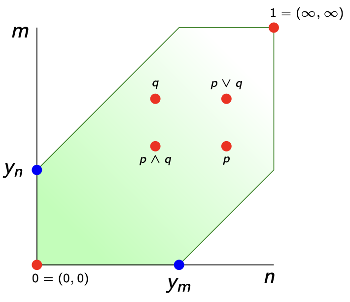
The set of all enriched presheaves $\widehat{V_d}$ has a lot of extra structure. It is a poset

$$p \leq q \qquad \text{iff} \qquad \forall n \in V : p(n) \leq q(n)$$

with minimal element $0 : \forall n \in V, 0(n)=0$, and maximal element $1 : \forall n \in V, 1(n)=\infty$.

It is even a lattice with $p \vee q(n) = max(p(n),q(n))$ and $p \wedge q(n)=min(p(n),q(n))$. It is easy to check that $p \wedge q$ and $p \vee q$ are again enriched presheaves.

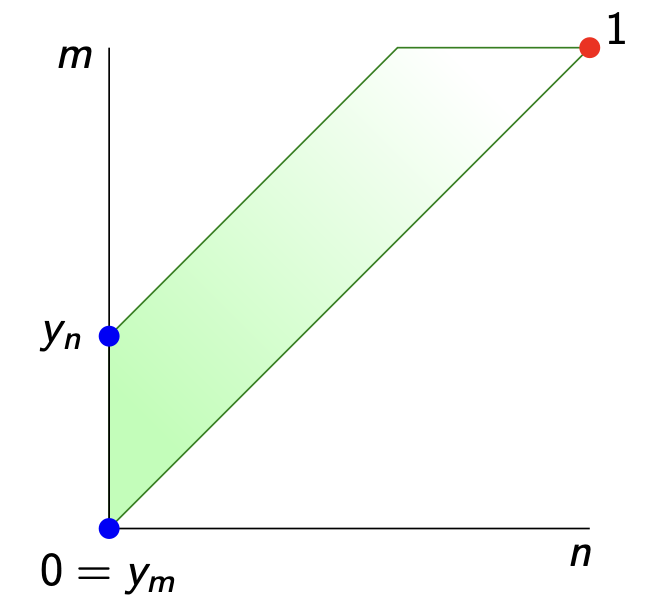
Here’s $\widehat{V_d}$ when the vault consists of just two notes $V=\{ m,n \}$ of non-zero distance to each other (whether symmetric or not) as a subset of $[0,\infty] \times [0,\infty]$.

This vault $\widehat{V_d}$ of all missing (and existing) notes is again enriched over $[0,\infty]$ via

$$\widehat{d} : \widehat{V_d} \times \widehat{V_d} \rightarrow [0,\infty] \qquad \widehat{d}(p,q) = max(0,\underset{n \in V}{sup} (q(n)-p(n)))$$

The triangle inequality follows because the definition of $\widehat{d}(p,q)$ is equivalent to $\forall m \in V : \widehat{d}(p,q)+p(m) \geq q(m)$. Even if we start from a symmetric distance function $d$ on $V$, it is clear that this extended distance $\widehat{d}$ on $\widehat{V_d}$ is far from symmetric. The Yoneda map

$$y : V_d \rightarrow \widehat{V_d} \qquad n \mapsto y_n$$

is an isometry and the enriched version of the Yoneda lemma says that for all $p \in \widehat{V_d}$

$$p(n) = \widehat{d}(y_n,p)$$

Indeed, taking $m=n$ in $\widehat{d}(y_n,f)+y_n(m) \geq p(m)$ gives $\widehat{d}(y_n,p) \geq p(n)$. Conversely,
from the presheaf condition $d(m,n)+p(n) \geq p(m)$ for all $m,n$ follows

$$p(n) \geq max(0,\underset{m \in V}{sup}(p(m)-d(m,n)) = \widehat{d}(y_n,p)$$

In his paper Taking categories seriously, Bill Lawvere suggested to consider enriched presheaves $p \in \widehat{V_d}$ as ‘refined’ closed set of the vault-space $V_d$.

For every subset of notes $X \subset V$ we can consider the presheaf (use triangle inequality)

$$p_X : V \rightarrow [0,\infty] \qquad m \mapsto \underset{n \in X}{inf}~d(m,n)$$

then its zero set $Z(p_X) = \{ m \in V~:~p_X(m)=0 \}$ can be thought of as the closure of $X$, and the collection of all such closed subsets define a topology on $V$.

In our simple example of the two note vault $V=\{ m,n \}$ this is just the discrete topology, but we can get more interesting spaces. If $d(n,m)=0$ but $d(m,n) > 0$

we get the Sierpinski space: $n$ is the only closed point, and lies in the closure of $m$. Of course, if your vault contains thousands of notes, you might get more interesting topologies.

In the special case when $V_d$ is a poset-category, as was the case in the shape of languages post, this topology is the down-set (or up-set) topology.

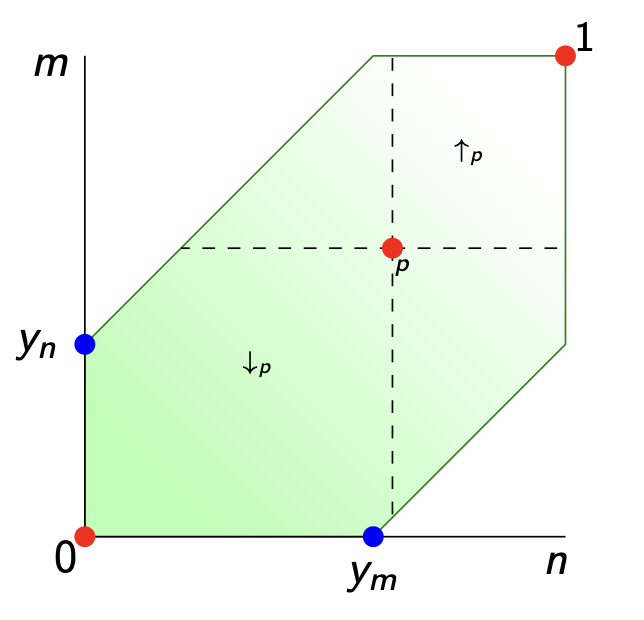
Now, what is this topology when you start with the Lawvere-space $\widehat{V_d}$? From the definitions we see that

$$\widehat{d}(p,q) = 0 \quad \text{iff} \quad \forall n \in V~:~p(n) \geq q(n) \quad \text{iff} \quad p \geq q$$

So, all presheaves in the up-set $\uparrow_p$ lie in the closure of $p$, and $p$ lies in the closure of all everything in the down-set $\downarrow_p$ of $p$. So, this time the topology has as its closed sets all down-sets of the poset $\widehat{V_d}$.

What’s missing is a good definition for the implication $p \Rightarrow q$ between two enriched presheaves $p,q \in \widehat{V_d}$. In An enriched category theory of language: from syntax to semantics it is said that this should be, perhaps only to be used in their special poset situation (with adapted notations)

$$p \Rightarrow q : V \rightarrow [0,\infty] \qquad \text{where} \quad (p \Rightarrow q)(n) = \widehat{d}(y_n \wedge p,q)$$

but I can’t even show that this is a presheaf. I may be horribly wrong, but in their proof of this (lemma 5) they seem to use their lemma 4, but with the two factors swapped.

If you have suggestions, please let me know. And if you trow Kelly’s Basic concepts of enriched category theory at me, please add some guidelines on how to use it. I’m just a passer-by.

Probably, I should also read up on Isbell duality, as suggested by Lawvere in his paper Taking categories seriously, and worked out by Simon Willerton in Tight spans, Isbell completions and semi-tropical modules…

(tbc)

Previously in this series:

Next

The tropical brain forest

Stella Maris (Cormac McCarthy)

Published March 17, 2023 by lievenlb

This week, I was hit hard by synchronicity.

Lately, I’ve been reading up a bit on psycho-analysis, tried to get through Grothendieck’s La clef des songes (the key to dreams) and I’m in the process of writing a series of blogposts on how to construct a topos of the unconscious.

And then I read Cormac McCarthy‘s novels The passenger and Stella Maris, and got hit.

Stella Maris is set in 1972, when the math-prodigy Alicia Western, suffering from hallucinations, admits herself to a psychiatric hospital, carrying a plastic bag containing forty thousand dollars. The book consists entirely of dialogues, the transcripts of seven sessions with her psychiatrist Dr. Cohen (nomen est omen).

Alicia is a doctoral candidate at the University Of Chicago who got a scholarship to visit the IHES to work with Grothendieck on toposes.

During the psychiatric sessions, they talk on a wide variety of topics, including the nature of mathematics, quantum mechanics, music theory, dreams, and the unconscious (and its role in doing mathematics).

The core question is not how you do math but how does the unconscious do it. How it is that it’s demonstrably better at it than you are? You work on a problem and then you put it away for a while. But it doesnt go away. It reappears at lunch. Or while you’re taking a shower. It says: Take a look at this. What do you think? Then you wonder why the shower is cold. Or the soup. Is this doing math? I’m afraid it is. How is it doing it? We dont know. How does the unconscious do math? (page 99)

Before going to the IHES she had to send Grothendieck a paper (‘It was an explication of topos theory that I thought he probably hadn’t considered.’ page 136, and ‘while it proved three problems in topos theory it then set about dismantling the mechanism of the proofs.’ page 151). At the IHES ‘I met three men that I could talk to: Grothendieck, Deligne, and Oscar Zariski.’ (page 136).

I don’t know whether Zariski visited the IHES in the early 70ties, and while most historical allusions (to Grothendieck’s life, his role in Bourbaki etc.) are correct, Alicia mentions the ‘Langlands project’ (page 66) which may very well have been the talk of town at the IHES in 1972, but the mention of Witten ‘Grothendieck writes everything down. Witten nothing.’ (page 100) raised an eyebrow.

The book also contains these two nice attempts to capture some of the essence of topos theory:

When you get to topos theory you are at the edge of another universe.
You have found a place to stand where you can look back at the world from nowhere. It’s not just some gestalt. It’s fundamental. (page 13)

You asked me about Grothendieck. The topos theory he came up with is a witches’ brew of topology and algebra and mathematical logic.
It doesnt even have a clear identity. The power of the theory is still speculative. But it’s there.
You have a sense that it is waiting quietly with answers to questions that nobody has asked yet. (page 68)

I did read ‘The passenger’ first, which is probably better as then you’d know already some of the ghosts haunting Alicia, but it’s not a must if you are only interested in their discussions about the nature of mathematics. Be warned that it is a pretty dark book, better not read when you’re already feeling low, and it should come with a link to a suicide prevention line.

Here’s a more considered take on Stella Maris:

4 Comments

The enriched vault

Published March 10, 2023 by lievenlb

In the shape of languages we started from a collection of notes, made a poset of text-snippets from them, and turned this into an enriched category over the unit interval $[0,1]$, following the paper paper An enriched category theory of language: from syntax to semantics by Tai-Danae Bradley, John Terilla and Yiannis Vlassopoulos.

This allowed us to view the text-snippets as points in a Lawvere pseudoquasi metric space, and to define a ‘topos’ of enriched presheaves on it, including the Yoneda-presheaves containing semantic information of the snippets.

In the previous post we looked at ‘building a second brain’ apps, such as LogSeq and Obsidian, and hoped to use them to test the conjectured ‘topos of the unconscious’.

In Obsidian, a vault is a collection of notes (with their tags and other meta-data), together with all links between them.

The vault of the language-poset will have one note for every text-snipped, and have a link from note $n$ to note $m$ if $m$ is a text-fragment in $n$.

In their paper, Bradley, Terilla and Vlassopoulos use the enrichment structure where $\mu(n,m) \in [0,1]$ is the conditional probablity of the fragment $m$ to be extended to the larger text $n$.

Most Obsidian vaults are a lot more complicated, possibly having oriented cycles in their internal link structure.

Still, it is always possible to turn the notes of the vault into a category enriched over $[0,1]$, in multiple ways, depending on whether we want to focus on the internal link-structure or rather on the semantic similarity between notes, or any combination of these.

Let $X$ be a set of searchable data from your vault. Elements of $X$ may be

words contained in notes
in- or out-going links between notes
tags used
YAML-frontmatter
…

Assign a positive real number $r_x \geq 0$ to every $x \in X$. We see $r_x$ as the ‘relevance’ we attach to the search term $x$. So, it is possible to emphasise certain key-words or tags, find certain links more important than others, and so on.

For this relevance function $r : X \rightarrow \mathbb{R}_+$, we have a function defined on all subsets $Y$ of $X$

$$f_r~:~\mathcal{P}(X) \rightarrow \mathbb{R}_+ \qquad Y \mapsto f_r(Y) = \sum_{x \in Y} r_x$$

Take a note $n$ from the vault $V$ and let $X_n$ be the set of search terms from $X$ contained in $n$.

We can then define a (generalised) Jaccard distance for any pair of notes $n$ and $m$ in $V$:

$$ d_r(n,m) = \begin{cases}
0~\text{if $f_r(X_n \cup X_m)=0$} \\ 1-\frac{f_r(X_n \cap X_m)}{f_r(X_n \cup X_m)}~\text{otherwise} \end{cases}$$

This distance is symmetric, $d_r(n,n)=0$ for all notes $n$, and the crucial property is that it satisfies the triangle inequality, that is, for all triples of notes $l$, $m$ and $n$ we have

$$d_r(l,n) \leq d_r(l,m)+d_r(m,n)$$

For a proof in this generality see the paper A note on the triangle inequality for the Jaccard distance by Sven Kosub.

How does this help to make the vault $V$ into a category enriched over $[0,1]$?

The poset $([0,1],\leq)$ is the category with objects all numbers $a \in [0,1]$, and a unique morphism $a \rightarrow b$ between two numbers iff $a \leq b$. This category has limits (infs) and colimits (sups), has a monoidal structure $a \otimes b = a \times b$ with unit object $1$, and an internal hom

$$Hom_{[0,1]}(a,b) = (a,b) = \begin{cases} \frac{b}{a}~\text{if $b \leq a$} \\ 1~\text{otherwise} \end{cases}$$

We say that the vault is an enriched category over $[0,1]$ if for every pair of notes $n$ and $m$ we have a number $\mu(n,m) \in [0,1]$ satisfying for all notes $n$

$$\mu(n,n)=1~\quad~\text{and}~\quad~\mu(m,l) \times \mu(n,m) \leq \mu(n,l)$$

for all triples of notes $l,m$ and $n$.

Starting from any relevance function $r : X \rightarrow \mathbb{R}_+$ we define for every pair $n$ and $m$ of notes the distance function $d_r(m,n)$ satisfying the triangle inequality. If we now take

$$\mu_r(m,n) = e^{-d_r(m,n)}$$

then the triangle inequality translates for every triple of notes $l,m$ and $n$ into

$$\mu_r(m,l) \times \mu_r(n,m) \leq \mu_r(n,l)$$

That is, every relevance function makes $V$ into a category enriched over $[0,1]$.

Two simple relevance functions, and their corresponding distance and enrichment functions are available from Obsidian’s Graph Analysis community plugin.

To get structural information on the link-structure take as $X$ the set of all incoming and outgoing links in your vault, with relevance function the constant function $1$.

‘Jaccard’ in Graph Analysis computes for the current note $n$ the value of $1-d_r(n,m)$ for all notes $m$, so if this value is $a \in [0,1]$, then the corresponding enrichment value is $\mu_r(m,n)=e^{a-1}$.

To get semantic information on the similarity between notes, let $X$ be the set of all words in all notes and take again as relevance function the constant function $1$.

To access ‘BoW’ (Bags of Words) in Graph Analysis, you must first install the (non-community) NLP plugin which enables various types of natural language processing in the vault. The install is best done via the BRAT plugin (perhaps I’ll do a couple of posts on Obsidian someday).

If it gives for the current note $n$ the value $a$ for a note $m$, then again we can take as the enrichment structure $\mu_r(n,m)=e^{a-1}$.

Graph Analysis offers more functionality, and a good introduction is given in this clip:

Calculating the enrichment data for custom designed relevance functions takes a lot more work, but is doable. Perhaps I’ll return to this later.

Mathematically, it is probably more interesting to start with a given enrichment structure $\mu$ on the vault $V$, describe the category of all enriched presheaves $\widehat{V_{\mu}}$ and find out what we can do with it.

(tbc)

Previously in this series:

Next:

The super-vault of missing notes