Tag: representations

noncommutative F_un geometry (2)

Published October 17, 2008 by lievenlb

Last time we tried to generalize the Connes-Consani approach to commutative algebraic geometry over the field with one element $\mathbb{F}_1 $ to the noncommutative world by considering covariant functors

$N~:~\mathbf{groups} \rightarrow \mathbf{sets} $

which over $\mathbb{C} $ resp. $\mathbb{Z} $ become visible by a complex (resp. integral) algebra having suitable universal properties.

However, we didn’t specify what we meant by a complex noncommutative variety (resp. an integral noncommutative scheme). In particular, we claimed that the $\mathbb{F}_1 $-‘points’ associated to the functor

$D~:~\mathbf{groups} \rightarrow \mathbf{sets} \qquad G \mapsto G_2 \times G_3 $ (here $G_n $ denotes all elements of order $n $ of $G $)

were precisely the modular dessins d’enfants of Grothendieck, but didn’t give details. We’ll try to do this now.

For algebras over a field we follow the definition, due to Kontsevich and Soibelman, of so called “noncommutative thin schemes”. Actually, the thinness-condition is implicit in both Soule’s-approach as that of Connes and Consani : we do not consider R-points in general, but only those of rings R which are finite and flat over our basering (or field).

So, what is a noncommutative thin scheme anyway? Well, its a covariant functor (commuting with finite projective limits)

$\mathbb{X}~:~\mathbf{Alg}^{fd}_k \rightarrow \mathbf{sets} $

from finite-dimensional (possibly noncommutative) $k $-algebras to sets. Now, the usual dual-space operator gives an anti-equivalence of categories

$\mathbf{Alg}^{fd}_k \leftrightarrow \mathbf{Coalg}^{fd}_k \qquad A=C^* \leftrightarrow C=A^* $

so a thin scheme can also be viewed as a contra-variant functor (commuting with finite direct limits)

$\mathbb{X}~:~\mathbf{Coalg}^{fd}_k \rightarrow \mathbf{Sets} $

In particular, we are interested to associated to any {tex]k $-algebra $A $ its representation functor :

$\mathbf{rep}(A)~:~\mathbf{Coalg}^{fd}_k \rightarrow \mathbf{Sets} \qquad C \mapsto Alg_k(A,C^*) $

This may look strange at first sight, but $C^* $ is a finite dimensional algebra and any $n $-dimensional representation of $A $ is an algebra map $A \rightarrow M_n(k) $ and we take $C $ to be the dual coalgebra of this image.

Kontsevich and Soibelman proved that every noncommutative thin scheme $\mathbb{X} $ is representable by a $k $-coalgebra. That is, there exists a unique coalgebra $C_{\mathbb{X}} $ (which they call the coalgebra of ‘distributions’ of $\mathbb{X} $) such that for every finite dimensional $k $-algebra $B $ we have

$\mathbb{X}(B) = Coalg_k(B^*,C_{\mathbb{X}}) $

In the case of interest to us, that is for the functor $\mathbf{rep}(A) $ the coalgebra of distributions is Kostant’s dual coalgebra $A^o $. This is the not the full linear dual of $A $ but contains only those linear functionals on $A $ which factor through a finite dimensional quotient.

So? You’ve exchanged an algebra $A $ for some coalgebra $A^o $, but where’s the geometry in all this? Well, let’s look at the commutative case. Suppose $A= \mathbb{C}[X] $ is the coordinate ring of a smooth affine variety $X $, then its dual coalgebra looks like

$\mathbb{C}[X]^o = \oplus_{x \in X} U(T_x(X)) $

the direct sum of all universal (co)algebras of tangent spaces at points $x \in X $. But how do we get the variety out of this? Well, any coalgebra has a coradical (being the sun of all simple subcoalgebras) and in the case just mentioned we have

$corad(\mathbb{C}[X]^o) = \oplus_{x \in X} \mathbb{C} e_x $

so every point corresponds to a unique simple component of the coradical. In the general case, the coradical of the dual coalgebra $A^o $ is the direct sum of all simple finite dimensional representations of $A $. That is, the direct summands of the coalgebra give us a noncommutative variety whose points are the simple representations, and the remainder of the coalgebra of distributions accounts for infinitesimal information on these points (as do the tangent spaces in the commutative case).

In fact, it was a surprise to me that one can describe the dual coalgebra quite explicitly, and that $A_{\infty} $-structures make their appearance quite naturally. See this paper if you’re in for the details on this.

That settles the problem of what we mean by the noncommutative variety associated to a complex algebra. But what about the integral case? In the above, we used extensively the theory of Kostant-duality which works only for algebras over fields…

Well, not quite. In the case of $\mathbb{Z} $ (or more general, of Dedekind domains) one can repeat Kostant’s proof word for word provided one takes as the definition of the dual $\mathbb{Z} $-coalgebra
of an algebra (which is $\mathbb{Z} $-torsion free)

$A^o = { f~:~A \rightarrow \mathbb{Z}~:~A/Ker(f)~\text{is finitely generated and torsion free}~} $

(over general rings there may be also variants of this duality, as in Street’s book an Quantum groups). Probably lots of people have come up with this, but the only explicit reference I have is to the first paper I’ve ever written. So, also for algebras over $\mathbb{Z} $ we can define a suitable noncommutative integral scheme (the coradical approach accounts only for the maximal ideals rather than all primes, but somehow this is implicit in all approaches as we consider only thin schemes).

Fine! So, we can make sense of the noncommutative geometrical objects corresponding to the group-algebras $\mathbb{C} \Gamma $ and $\mathbb{Z} \Gamma $ where $\Gamma = PSL_2(\mathbb{Z}) $ is the modular group (the algebras corresponding to the $G \mapsto G_2 \times G_3 $-functor). But, what might be the points of the noncommutative scheme corresponding to $\mathbb{F}_1 \Gamma $???

Well, let’s continue the path cut out before. “Points” should correspond to finite dimensional “simple representations”. Hence, what are the finite dimensional simple $\mathbb{F}_1 $-representations of $\Gamma $? (Or, for that matter, of any group $G $)

Here we come back to Javier’s post on this : a finite dimensional $\mathbb{F}_1 $-vectorspace is a finite set. A $\Gamma $-representation on this set (of n-elements) is a group-morphism

$\Gamma \rightarrow GL_n(\mathbb{F}_1) = S_n $

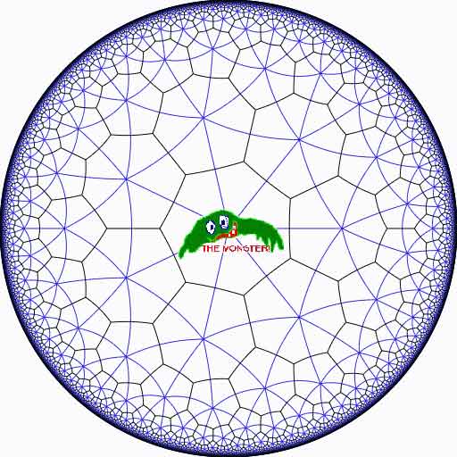
hence it gives a permutation representation of $\Gamma $ on this set. But then, if finite dimensional $\mathbb{F}_1 $-representations of $\Gamma $ are the finite permutation representations, then the simple ones are the transitive permutation representations. That is, the points of the noncommutative scheme corresponding to $\mathbb{F}_1 \Gamma $ are the conjugacy classes of subgroups $H \subset \Gamma $ such that $\Gamma/H $ is finite. But these are exactly the modular dessins d’enfants introduced by Grothendieck as I explained a while back elsewhere (see for example this post and others in the same series).

noncommutative F_un geometry (1)

Published October 13, 2008 by lievenlb

It is perhaps surprising that Alain Connes and Katia Consani, two icons of noncommutative geometry, restrict themselves to define commutative algebraic geometry over $\mathbb{F}_1 $, the field with one element.

My guess of why they stop there is as good as anyone’s. Perhaps they felt that there is already enough noncommutativity in Soule’s gadget-approach (the algebra $\mathcal{A}_X $ as in this post may very well be noncommutative). Perhaps they were only interested in the Bost-Connes system which can be entirely encoded in their commutative $\mathbb{F}_1 $-geometry. Perhaps they felt unsure as to what the noncommutative scheme of an affine noncommutative algebra might be. Perhaps …

Remains the fact that their approach screams for a noncommutative extension. Their basic object is a covariant functor

$N~:~\mathbf{abelian} \rightarrow \mathbf{sets} \qquad A \mapsto N(A) $

from finite abelian groups to sets, together with additional data to the effect that there is a unique minimal integral scheme associated to $N $. In a series of posts on the Connes-Consani paper (starting here) I took some care of getting rid of all scheme-lingo and rephrasing everything entirely into algebras. But then, this set-up can be extended verbatim to noncommuative $\mathbb{F}_1 $-geometry, which should start from a covariant functor

$N~:~\mathbf{groups} \rightarrow \mathbf{sets} $

from all finite groups to sets. Let’s recall quickly what the additional info should be making this functor a noncommutative (affine) F_un scheme :

There should be a finitely generated $\mathbb{C} $-algebra $R $ together with a natural transformation (the ‘evaluation’)

$e~:~N \rightarrow \mathbf{maxi}(R) \qquad N(G) \mapsto Hom_{\mathbb{C}-alg}(R, \mathbb{C} G) $

(both $R $ and the group-algebra $\mathbb{C} G $ may be noncommutative). The pair $(N, \mathbf{maxi}(R)) $ is then called a gadget and there is an obvious notion of ‘morphism’ between gadgets.

The crucial extra ingredient is an affine $\mathbb{Z} $-algebra (possibly noncommutative) $S $
such that $N $ is a subfunctor of $\mathbf{mini}(S)~:~G \mapsto Hom_{\mathbb{Z}-alg}(S,\mathbb{Z} G) $ together with the following universal property :

any affine $\mathbb{Z} $-algebra $T $ having a gadget-morphism $~(N,\mathbf{maxi}(R)) \rightarrow (\mathbf{mini}(T),\mathbf{maxi}(T \otimes_{\mathbb{Z}} \mathbb{C})) $ comes from a $\mathbb{Z} $-algebra morphism $T \rightarrow S $. (If this sounds too cryptic for you, please read the series on C-C mentioned before).

So, there is no problem in defining noncommutative affine F_un-schemes. However, as with any generalization, this only makes sense provided (a) we get something new and (b) we have interesting examples, not covered by the restricted theory.

At first sight we do not get something new as in the only example we did in the C-C-series (the forgetful functor) it is easy to prove (using the same proof as given in this post) that the forgetful-functor $\mathbf{groups} \rightarrow \mathbf{sets} $ still has as its integral form the integral torus $\mathbb{Z}[x,x^{-1}] $. However, both theories quickly diverge beyond this example.

For example, consider the functor

$\mathbf{groups} \rightarrow \mathbf{sets} \qquad G \mapsto G \times G $

Then, if we restrict to abelian finite groups $\mathbf{abelian} $ it is easy to see (again by a similar argument) that the two-dimensional integer torus $\mathbb{Z}[x,y,x^{-1},y^{-1}] $ is the correct integral form. However, this algebra cannot be the correct form for the functor on the category of all finite groups as any $\mathbb{Z} $-algebra map $\phi~:~\mathbb{Z}[x,y,x^{-1},y^{-1}] \rightarrow \mathbb{Z} G $ determines (and is determined by) a pair of commuting units in $\mathbb{Z} G $, so the above functor can not be a subfunctor if we allow non-Abelian groups.

But then, perhaps there isn’t a minimal integral $\mathbb{Z} $-form for this functor? Well, yes there is. Take the free group in two letters (that is, all words in noncommuting $x,y,x^{-1} $ and $y^{-1} $ satisfying only the trivial cancellation laws between a letter and its inverse), then the corresponding integral group-algebra $\mathbb{Z} \mathcal{F}_2 $ does the trick.

Again, the proof-strategy is the same. Given a gadget-morphism we have an algebra map $f~:~T \mapsto \mathbb{C} \mathcal{F}_2 $ and we have to show, using the universal property that the image of $T $ is contained in the integral group-algebra $\mathbb{Z} \mathcal{F}_2 $. Take a generator
$z $ of $T $ then the degree of the image $f(z) $ is bounded say by $d $ and we can always find a subgroup $H \subset \mathcal{F}_2 $ such that $\mathcal{F}_2/H $ is a fnite group and the quotient map $\mathbb{C} \mathcal{F}_2 \rightarrow \mathbb{C} \mathcal{F}_2/H $ is injective on the subspace spanned by all words of degree strictly less than $d+1 $. Then, the usual diagram-chase finishes the proof.

What makes this work is that the free group $\mathcal{F}_2 $ has ‘enough’ subgroups of finite index, a property it shares with many interesting discrete groups. Whence the blurb-message :

if the integers $\mathbb{Z} $ see a discrete group $\Gamma $, then the field $\mathbb{F}_1 $ sees its profinite completion $\hat{\Gamma} = \underset{\leftarrow}{lim}~\Gamma/ H $

So, yes, we get something new by extending the Connes-Consani approach to the noncommutative world, but do we have interesting examples? As “interesting” is a subjective qualification, we’d better invoke the authority-argument.

Alexander Grothendieck (sitting on the right, manifestly not disputing a vacant chair with Jean-Pierre Serre, drinking on the left (a marvelous picture taken by F. Hirzebruch in 1958)) was pushing the idea that profinite completions of arithmetical groups were useful in the study of the absolute Galois group $Gal(\overline{\mathbb{Q}}/\mathbb{Q}) $, via his theory of dessins d’enfants (children;s drawings).

In a previous life, I’ve written a series of posts on dessins d’enfants, so I’ll restrict here to the basics. A smooth projective $\overline{\mathbb{Q}} $-curve $X $ has a Belyi-map $X \rightarrow \mathbb{P}^1_{\overline{\mathbb{Q}}} $ ramified only in three points ${ 0,1,\infty } $. The “drawing” corresponding to $X $ is a bipartite graph, drawn on the Riemann surface $X_{\mathbb{C}} $ obtained by lifting the unit interval $[0,1] $ to $X $. As the absolute Galois group acts on all such curves (and hence on their corresponding drawings), the action of it on these dessins d’enfants may give us a way into the multiple mysteries of the absolute Galois group.

In his “Esquisse d’un programme” (Sketch of a program if you prefer to read it in English) he writes :

“C’est ainsi que mon attention s’est portée vers ce que j’ai appelé depuis la “géométrie algêbrique anabélienne”, dont le point de départ est justement une étude (pour le moment limitée à la caractéristique zéro) de l’action de groupe de Galois “absolus” (notamment les groupes $Gal(\overline{K}/K) $, ou $K $ est une extension de type fini du corps premier) sur des groupes fondamentaux géométriques (profinis) de variétés algébriques (définies sur $K $), et plus particulièrement (rompant avec une tradition bien enracinée) des groupes fondamentaux qui sont trés éloignés des groupes abéliens (et que pour cette raison je nomme “anabéliens”). Parmi ces groupes, et trés proche du groupe $\hat{\pi}_{0,3} $, il y a le compactifié profini du groupe modulaire $SL_2(\mathbb{Z}) $, dont le quotient par le centre $\pm 1 $ contient le précédent comme sous-groupe de congruence mod 2, et peut s’interpréter d’ailleurs comme groupe “cartographique” orienté, savoir celui qui classifie les cartes orientées triangulées (i.e. celles dont les faces des triangles ou des monogones).”

and a bit further, he writes :

“L’élément de structure de $SL_2(\mathbb{Z}) $ qui me fascine avant tout, est bien sur l’action extérieure du groupe de Galois $Gal(\overline{\mathbb{Q}}/\mathbb{Q}) $ sur le compactifié profini. Par le théorème de Bielyi, prenant les compactifiés profinis de sous-groupes d’indice fini de $SL_2(\mathbb{Z}) $, et l’action extérieure induite (quitte à passer également à un sous-groupe overt de $Gal(\overline{\mathbb{Q}},\mathbb{Q}) $), on trouve essentiellement les groupes fondamentaux de toutes les courbes algébriques définis sur des corps de nombres $K $, et l’action extérieure de $Gal(\overline{K}/K) $ dessus.”

So, is there a noncommutative affine variety over $\mathbb{F}_1 $ of which the unique minimal integral model is the integral group algebra of the modular group $\mathbb{Z} \Gamma $ (with $\Gamma = PSL_2(\mathbb{Z}) $? Yes, here it is

$N_{\Gamma}~:~\mathbf{groups} \rightarrow \mathbf{sets} \qquad G \mapsto G_2 \times G_3 $

where $G_n $ is the set of all elements of order $n $ in $G $. The reason behind this is that the modular group is the free group product $C_2 \ast C_3 $.

Fine, you may say, but all this is just algebra. Where is the noncommutative complex variety or the noncommutative integral scheme in all this? Well, we can introduce them too but as this post is already 1300 words long, I’ll better leave this for another time. In case you cannot stop thinking about it, here’s the short answer.

The complex noncommutative variety has as its ‘points’ all finite dimensional simple complex representations of the modular group, and the ‘points’ of the noncommutative $\mathbb{F}_1 $-scheme are exactly the (modular) dessins d’enfants…

what does the monster see?

Published July 16, 2008 by lievenlb

The Monster is the largest of the 26 sporadic simple groups and has order

808 017 424 794 512 875 886 459 904 961 710 757 005 754 368 000 000 000

= 2^46 3^20 5^9 7^6 11^2 13^3 17 19 23 29 31 41 47 59 71.

It is not so much the size of its order that makes it hard to do actual calculations in the monster, but rather the dimensions of its smallest non-trivial irreducible representations (196 883 for the smallest, 21 296 876 for the next one, and so on).

In characteristic two there is an irreducible representation of one dimension less (196 882) which appears to be of great use to obtain information. For example, Robert Wilson used it to prove that The Monster is a Hurwitz group. This means that the Monster is generated by two elements g and h satisfying the relations

$g^2 = h^3 = (gh)^7 = 1 $

Geometrically, this implies that the Monster is the automorphism group of a Riemann surface of genus g satisfying the Hurwitz bound 84(g-1)=#Monster. That is,

g=9619255057077534236743570297163223297687552000000001=42151199 * 293998543 * 776222682603828537142813968452830193

Or, in analogy with the Klein quartic which can be constructed from 24 heptagons in the tiling of the hyperbolic plane, there is a finite region of the hyperbolic plane, tiled with heptagons, from which we can construct this monster curve by gluing the boundary is a specific way so that we get a Riemann surface with exactly 9619255057077534236743570297163223297687552000000001 holes. This finite part of the hyperbolic tiling (consisting of #Monster/7 heptagons) we’ll call the empire of the monster and we’d love to describe it in more detail.

Look at the half-edges of all the heptagons in the empire (the picture above learns that every edge in cut in two by a blue geodesic). They are exactly #Monster such half-edges and they form a dessin d’enfant for the monster-curve.

If we label these half-edges by the elements of the Monster, then multiplication by g in the monster interchanges the two half-edges making up a heptagonal edge in the empire and multiplication by h in the monster takes a half-edge to the one encountered first by going counter-clockwise in the vertex of the heptagonal tiling. Because g and h generated the Monster, the dessin of the empire is just a concrete realization of the monster.

Because g is of order two and h is of order three, the two permutations they determine on the dessin, gives a group epimorphism $C_2 \ast C_3 = PSL_2(\mathbb{Z}) \rightarrow \mathbb{M} $ from the modular group $PSL_2(\mathbb{Z}) $ onto the Monster-group.

In noncommutative geometry, the group-algebra of the modular group $\mathbb{C} PSL_2 $ can be interpreted as the coordinate ring of a noncommutative manifold (because it is formally smooth in the sense of Kontsevich-Rosenberg or Cuntz-Quillen) and the group-algebra of the Monster $\mathbb{C} \mathbb{M} $ itself corresponds in this picture to a finite collection of ‘points’ on the manifold. Using this geometric viewpoint we can now ask the question What does the Monster see of the modular group?

To make sense of this question, let us first consider the commutative equivalent : what does a point P see of a commutative variety X?

Evaluation of polynomial functions in P gives us an algebra epimorphism $\mathbb{C}[X] \rightarrow \mathbb{C} $ from the coordinate ring of the variety $\mathbb{C}[X] $ onto $\mathbb{C} $ and the kernel of this map is the maximal ideal $\mathfrak{m}_P $ of
$\mathbb{C}[X] $ consisting of all functions vanishing in P.

Equivalently, we can view the point $P= \mathbf{spec}~\mathbb{C}[X]/\mathfrak{m}_P $ as the scheme corresponding to the quotient $\mathbb{C}[X]/\mathfrak{m}_P $. Call this the 0-th formal neighborhood of the point P.

This sounds pretty useless, but let us now consider higher-order formal neighborhoods. Call the affine scheme $\mathbf{spec}~\mathbb{C}[X]/\mathfrak{m}_P^{n+1} $ the n-th forml neighborhood of P, then the first neighborhood, that is with coordinate ring $\mathbb{C}[X]/\mathfrak{m}_P^2 $ gives us tangent-information. Alternatively, it gives the best linear approximation of functions near P.
The second neighborhood $\mathbb{C}[X]/\mathfrak{m}_P^3 $ gives us the best quadratic approximation of function near P, etc. etc.

These successive quotients by powers of the maximal ideal $\mathfrak{m}_P $ form a system of algebra epimorphisms

$\ldots \frac{\mathbb{C}[X]}{\mathfrak{m}_P^{n+1}} \rightarrow \frac{\mathbb{C}[X]}{\mathfrak{m}_P^{n}} \rightarrow \ldots \ldots \rightarrow \frac{\mathbb{C}[X]}{\mathfrak{m}_P^{2}} \rightarrow \frac{\mathbb{C}[X]}{\mathfrak{m}_P} = \mathbb{C} $

and its inverse limit $\underset{\leftarrow}{lim}~\frac{\mathbb{C}[X]}{\mathfrak{m}_P^{n}} = \hat{\mathcal{O}}_{X,P} $ is the completion of the local ring in P and contains all the infinitesimal information (to any order) of the variety X in a neighborhood of P. That is, this completion $\hat{\mathcal{O}}_{X,P} $ contains all information that P can see of the variety X.

In case P is a smooth point of X, then X is a manifold in a neighborhood of P and then this completion
$\hat{\mathcal{O}}_{X,P} $ is isomorphic to the algebra of formal power series $\mathbb{C}[[ x_1,x_2,\ldots,x_d ]] $ where the $x_i $ form a local system of coordinates for the manifold X near P.

Right, after this lengthy recollection, back to our question what does the monster see of the modular group? Well, we have an algebra epimorphism

$\pi~:~\mathbb{C} PSL_2(\mathbb{Z}) \rightarrow \mathbb{C} \mathbb{M} $

and in analogy with the commutative case, all information the Monster can gain from the modular group is contained in the $\mathfrak{m} $-adic completion

$\widehat{\mathbb{C} PSL_2(\mathbb{Z})}_{\mathfrak{m}} = \underset{\leftarrow}{lim}~\frac{\mathbb{C} PSL_2(\mathbb{Z})}{\mathfrak{m}^n} $

where $\mathfrak{m} $ is the kernel of the epimorphism $\pi $ sending the two free generators of the modular group $PSL_2(\mathbb{Z}) = C_2 \ast C_3 $ to the permutations g and h determined by the dessin of the pentagonal tiling of the Monster’s empire.

As it is a hopeless task to determine the Monster-empire explicitly, it seems even more hopeless to determine the kernel $\mathfrak{m} $ let alone the completed algebra… But, (surprise) we can compute $\widehat{\mathbb{C} PSL_2(\mathbb{Z})}_{\mathfrak{m}} $ as explicitly as in the commutative case we have $\hat{\mathcal{O}}_{X,P} \simeq \mathbb{C}[[ x_1,x_2,\ldots,x_d ]] $ for a point P on a manifold X.

Here the details : the quotient $\mathfrak{m}/\mathfrak{m}^2 $ has a natural structure of $\mathbb{C} \mathbb{M} $-bimodule. The group-algebra of the monster is a semi-simple algebra, that is, a direct sum of full matrix-algebras of sizes corresponding to the dimensions of the irreducible monster-representations. That is,

$\mathbb{C} \mathbb{M} \simeq \mathbb{C} \oplus M_{196883}(\mathbb{C}) \oplus M_{21296876}(\mathbb{C}) \oplus \ldots \ldots \oplus M_{258823477531055064045234375}(\mathbb{C}) $

with exactly 194 components (the number of irreducible Monster-representations). For any $\mathbb{C} \mathbb{M} $-bimodule $M $ one can form the tensor-algebra

$T_{\mathbb{C} \mathbb{M}}(M) = \mathbb{C} \mathbb{M} \oplus M \oplus (M \otimes_{\mathbb{C} \mathbb{M}} M) \oplus (M \otimes_{\mathbb{C} \mathbb{M}} M \otimes_{\mathbb{C} \mathbb{M}} M) \oplus \ldots \ldots $

and applying the formal neighborhood theorem for formally smooth algebras (such as $\mathbb{C} PSL_2(\mathbb{Z}) $) due to Joachim Cuntz (left) and Daniel Quillen (right) we have an isomorphism of algebras

$\widehat{\mathbb{C} PSL_2(\mathbb{Z})}_{\mathfrak{m}} \simeq \widehat{T_{\mathbb{C} \mathbb{M}}(\mathfrak{m}/\mathfrak{m}^2)} $

where the right-hand side is the completion of the tensor-algebra (at the unique graded maximal ideal) of the $\mathbb{C} \mathbb{M} $-bimodule $\mathfrak{m}/\mathfrak{m}^2 $, so we’d better describe this bimodule explicitly.

Okay, so what’s a bimodule over a semisimple algebra of the form $S=M_{n_1}(\mathbb{C}) \oplus \ldots \oplus M_{n_k}(\mathbb{C}) $? Well, a simple S-bimodule must be either (1) a factor $M_{n_i}(\mathbb{C}) $ with all other factors acting trivially or (2) the full space of rectangular matrices $M_{n_i \times n_j}(\mathbb{C}) $ with the factor $M_{n_i}(\mathbb{C}) $ acting on the left, $M_{n_j}(\mathbb{C}) $ acting on the right and all other factors acting trivially.

That is, any S-bimodule can be represented by a quiver (that is a directed graph) on k vertices (the number of matrix components) with a loop in vertex i corresponding to each simple factor of type (1) and a directed arrow from i to j corresponding to every simple factor of type (2).

That is, for the Monster, the bimodule $\mathfrak{m}/\mathfrak{m}^2 $ is represented by a quiver on 194 vertices and now we only have to determine how many loops and arrows there are at or between vertices.

Using Morita equivalences and standard representation theory of quivers it isn’t exactly rocket science to determine that the number of arrows between the vertices corresponding to the irreducible Monster-representations $S_i $ and $S_j $ is equal to

$dim_{\mathbb{C}}~Ext^1_{\mathbb{C} PSL_2(\mathbb{Z})}(S_i,S_j)-\delta_{ij} $

Now, I’ve been wasting a lot of time already here explaining what representations of the modular group have to do with quivers (see for example here or some other posts in the same series) and for quiver-representations we all know how to compute Ext-dimensions in terms of the Euler-form applied to the dimension vectors.

Right, so for every Monster-irreducible $S_i $ we have to determine the corresponding dimension-vector $~(a_1,a_2;b_1,b_2,b_3) $ for the quiver

$\xymatrix{ & & & &
\vtx{b_1} \\ \vtx{a_1} \ar[rrrru]^(.3){B_{11}} \ar[rrrrd]^(.3){B_{21}}
\ar[rrrrddd]_(.2){B_{31}} & & & & \\ & & & & \vtx{b_2} \\ \vtx{a_2}
\ar[rrrruuu]_(.7){B_{12}} \ar[rrrru]_(.7){B_{22}}
\ar[rrrrd]_(.7){B_{23}} & & & & \\ & & & & \vtx{b_3}} $

Now the dimensions $a_i $ are the dimensions of the +/-1 eigenspaces for the order 2 element g in the representation and the $b_i $ are the dimensions of the eigenspaces for the order 3 element h. So, we have to determine to which conjugacy classes g and h belong, and from Wilson’s paper mentioned above these are classes 2B and 3B in standard Atlas notation.

So, for each of the 194 irreducible Monster-representations we look up the character values at 2B and 3B (see below for the first batch of those) and these together with the dimensions determine the dimension vector $~(a_1,a_2;b_1,b_2,b_3) $.

For example take the 196883-dimensional irreducible. Its 2B-character is 275 and the 3B-character is 53. So we are looking for a dimension vector such that $a_1+a_2=196883, a_1-275=a_2 $ and $b_1+b_2+b_3=196883, b_1-53=b_2=b_3 $ giving us for that representation the dimension vector of the quiver above $~(98579,98304,65663,65610,65610) $.

Okay, so for each of the 194 irreducibles $S_i $ we have determined a dimension vector $~(a_1(i),a_2(i);b_1(i),b_2(i),b_3(i)) $, then standard quiver-representation theory asserts that the number of loops in the vertex corresponding to $S_i $ is equal to

$dim(S_i)^2 + 1 – a_1(i)^2-a_2(i)^2-b_1(i)^2-b_2(i)^2-b_3(i)^2 $

and that the number of arrows from vertex $S_i $ to vertex $S_j $ is equal to

$dim(S_i)dim(S_j) – a_1(i)a_1(j)-a_2(i)a_2(j)-b_1(i)b_1(j)-b_2(i)b_2(j)-b_3(i)b_3(j) $

This data then determines completely the $\mathbb{C} \mathbb{M} $-bimodule $\mathfrak{m}/\mathfrak{m}^2 $ and hence the structure of the completion $\widehat{\mathbb{C} PSL_2}_{\mathfrak{m}} $ containing all information the Monster can gain from the modular group.

But then, one doesn’t have to go for the full regular representation of the Monster. Any faithful permutation representation will do, so we might as well go for the one of minimal dimension.

That one is known to correspond to the largest maximal subgroup of the Monster which is known to be a two-fold extension $2.\mathbb{B} $ of the Baby-Monster. The corresponding permutation representation is of dimension 97239461142009186000 and decomposes into Monster-irreducibles

$S_1 \oplus S_2 \oplus S_4 \oplus S_5 \oplus S_9 \oplus S_{14} \oplus S_{21} \oplus S_{34} \oplus S_{35} $

(in standard Atlas-ordering) and hence repeating the arguments above we get a quiver on just 9 vertices! The actual numbers of loops and arrows (I forgot to mention this, but the quivers obtained are actually symmetric) obtained were found after laborious computations mentioned in this post and the details I’ll make avalable here.

Anyone who can spot a relation between the numbers obtained and any other part of mathematics will obtain quantities of genuine (ie. non-Inbev) Belgian beer…

8 Comments