“Ne pleure pas, Alfred ! J’ai besoin de tout mon courage pour mourir à vingt ans!”
We all remember the last words of Evariste Galois to his brother Alfred. Lesser known are the mathematical results contained in his last letter, written to his friend Auguste Chevalier, on the eve of his fatal duel. Here the final sentences :
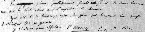
Tu prieras publiquement Jacobi ou Gauss de donner leur avis non sur la verite, mais sur l’importance des theoremes.
Apres cela il se trouvera, j’espere, des gens qui trouvent leur profis a dechiffrer tout ce gachis.
Je t’embrasse avec effusion.
E. Galois, le 29 Mai 1832
A major result contained in this letter concerns the groups $L_2(p)=PSL_2(\mathbb{F}_p) $, that is the group of $2 \times 2 $ matrices with determinant equal to one over the finite field $\mathbb{F}_p $ modulo its center. $L_2(p) $ is known to be simple whenever $p \geq 5 $. Galois writes that $L_2(p) $ cannot have a non-trivial permutation representation on fewer than $p+1 $ symbols whenever $p > 11 $ and indicates the transitive permutation representation on exactly $p $ symbols in the three ‘exceptional’ cases $p=5,7,11 $.
Let $\alpha = \begin{bmatrix} 1 & 1 \\ 0 & 1 \end{bmatrix} $ and consider for $p=5,7,11 $ the involutions on $\mathbb{P}^1_{\mathbb{F}_p} = \mathbb{F}_p \cup { \infty } $ (on which $L_2(p) $ acts via Moebius transformations)
$\pi_5 = (0,\infty)(1,4)(2,3) \quad \pi_7=(0,\infty)(1,3)(2,6)(4,5) \quad \pi_{11}=(0,\infty)(1,6)(3,7)(9,10)(5,8)(4,2) $
(in fact, Galois uses the involution $~(0,\infty)(1,2)(3,6)(4,8)(5,10)(9,7) $ for $p=11 $), then $L_2(p) $ leaves invariant the set consisting of the $p $ involutions $\Pi = { \alpha^{-i} \pi_p \alpha^i~:~1 \leq i \leq p } $. After mentioning these involutions Galois merely writes :
Ainsi pour le cas de $p=5,7,11 $, l’equation modulaire s’abaisse au degre p.
En toute rigueur, cette reduction n’est pas possible dans les cas plus eleves.
Alternatively, one can deduce these permutation representation representations from group isomorphisms. As $L_2(5) \simeq A_5 $, the alternating group on 5 symbols, $L_2(5) $ clearly acts transitively on 5 symbols.
 Similarly, for $p=7 $ we have $L_2(7) \simeq L_3(2) $ and so the group acts as automorphisms on the projective plane over the field on two elements $\mathbb{P}^2_{\mathbb{F}_2} $ aka the Fano plane, as depicted on the left.
This finite projective plane has 7 points and 7 lines and $L_3(2) $ acts transitively on them.
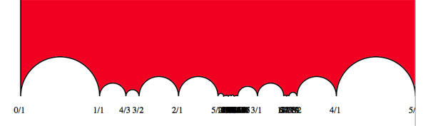
For $p=11 $ the geometrical object is a bit more involved. The set of non-squares in $\mathbb{F}_{11} $ is
${ 1,3,4,5,9 } $
and if we translate this set using the additive structure in $\mathbb{F}_{11} $ one obtains the following 11 five-element sets
${ 1,3,4,5,9 }, { 2,4,5,6,10 }, { 3,5,6,7,11 }, { 1,4,6,7,8 }, { 2,5,7,8,9 }, { 3,6,8,9,10 }, $
$ { 4,7,9,10,11 }, { 1,5,8,10,11 }, { 1,2,6,9,11 }, { 1,2,3,7,10 }, { 2,3,4,8,11 } $
and if we regard these sets as ‘lines’ we see that two distinct lines intersect in exactly 2 points and that any two distinct points lie on exactly two ‘lines’. That is, intersection sets up a bijection between the 55-element set of all pairs of distinct points and the 55-element set of all pairs of distinct ‘lines’. This is called the biplane geometry.
The subgroup of $S_{11} $ (acting on the eleven elements of $\mathbb{F}_{11} $) stabilizing this set of 11 5-element sets is precisely the group $L_2(11) $ giving the permutation representation on 11 objects.
An alternative statement of Galois’ result is that for $p > 11 $ there is no subgroup of $L_2(p) $ complementary to the cyclic subgroup
$C_p = { \begin{bmatrix} 1 & x \\ 0 & 1 \end{bmatrix}~:~x \in \mathbb{F}_p } $
That is, there is no subgroup such that set-theoretically $L_2(p) = F \times C_p $ (note this is of courese not a group-product, all it says is that any element can be written as $g=f.c $ with $f \in F, c \in C_p $.
However, in the three exceptional cases we do have complementary subgroups. In fact, set-theoretically we have
$L_2(5) = A_4 \times C_5 \qquad L_2(7) = S_4 \times C_7 \qquad L_2(11) = A_5 \times C_{11} $
and it is a truly amazing fact that the three groups appearing are precisely the three Platonic groups!
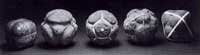 Recall that here are 5 Platonic (or Scottish) solids coming in three sorts when it comes to rotation-automorphism groups : the tetrahedron (group $A_4 $), the cube and octahedron (group $S_4 $) and the dodecahedron and icosahedron (group $A_5 $). The “4” in the cube are the four body diagonals and the “5” in the dodecahedron are the five inscribed cubes.
That is, our three ‘exceptional’ Galois-groups correspond to the three Platonic groups, which in turn correspond to the three exceptional Lie algebras $E_6,E_7,E_8 $ via McKay correspondence (wrt. their 2-fold covers). Maybe I’ll detail this latter connection another time. It sure seems that surprises often come in triples…
Finally, it is well known that $L_2(5) \simeq A_5 $ is the automorphism group of the icosahedron (or dodecahedron) and that $L_2(7) $ is the automorphism group of the Klein quartic.
So, one might ask : is there also a nice curve connected with the third group $L_2(11) $? Rumour has it that this is indeed the case and that the curve in question has genus 70… (to be continued).
Reference
Bertram Kostant, “The graph of the truncated icosahedron and the last letter of Galois”
Leave a Comment