Tag: Penrose tiling

de Bruijn’s pentagrids

Published March 11, 2021 by lievenlb

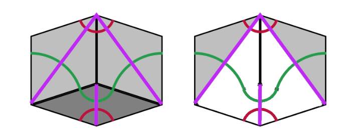
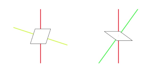
In a Rhombic tiling (aka a Penrose P3 tiling) we can identify five ribbons.

Opposite sides of a rhomb are parallel. We may form a ribbon by attaching rhombs along opposite sides. There are five directions taken by sides, so there are five families of ribbons that do not intersect, determined by the side directions.

Every ribbon determines a skeleton curve through the midpoints of opposite sides of the rhombs. If we straighten these skeleton curves we get a de Bruijn’s pentagrid.

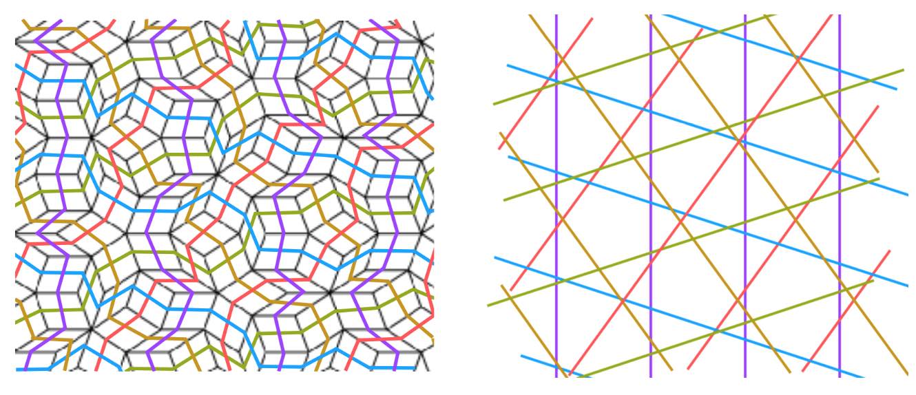
A pentagrid is a grid of the plane consisting of five families of parallel lines, at angles multiples of $72^o = 360^o/5$, and with each family consisting of parallel lines with a spacing given by a number $\gamma_i$ for $0 \leq i \leq 4$, satisfying
\[
\gamma_0+\gamma_1+\gamma_2+\gamma_3+\gamma_4=0 \]

The points of the plane in the $j$-th family of the pentagrid are
\[
\{ \vec{x} \in \mathbb{R}^2~|~\vec{x}.\vec{v}_j + \gamma_j \in \mathbb{Z} \} \]
where $\vec{v}_j = \zeta^j = (cos(2 \pi j/5),sin(2 \pi j/5))$.

A pentagrid is regular if no point in $\mathbb{R}^2$ belongs to more than two of the five grids. For almost all choices $\gamma_0,\dots,\gamma_4$ the corresponding pentagrid is regular. The pentagrid coordinates of a point $\vec{x} \in \mathbb{R}^2$ are the five integers $(K_0(\vec{x}),\dots,K_4(\vec{x}) \in \mathbb{Z}^5$ defined by
\[
K_j(\vec{x}) = \lceil \vec{x}.\vec{v}_j + \gamma_j \rceil \]
with $\lceil r \rceil$ the smallest integer greater of equal to $r$, and clearly the function $K_j(\vec{x})$ is constant in regions between the $j$-th grid lines.

With these pentagrid-coordinates one can associate a vertex to any point $\vec{x} \in \mathbb{R}^2$
\[
V(\vec{x}) = \sum_{j=0}^4 K_j(\vec{x}) \vec{v}_j \]
which is constant in regions between grid lines.

Here’s de Bruijn‘s result:

For $\vec{x}$ running over $\mathbb{R}^2$, the vertices $V(\vec{x})$ coming from a pentagrid determine a Rhombic tiling of the plane. Even better, every Rhombic tiling comes from a pentagrid.

We’ll prove this for regular pentagrids (the singular case follows from a small deformation).

Any intersection point $\vec{x}_0$ of the pentagrid belongs to exactly two families of parallel lines, so we have two integers $r$ and $s$ with $0 \leq r < s \leq 4$ and integers $k_r,k_s \in \mathbb{Z}$ such that $\vec{x}_0$ is determined by the equations \[ \begin{cases} \vec{x}.\vec{v}_r + \gamma_r = k_r \\ \vec{x}.\vec{v}_s + \gamma_s = k_s \end{cases} \] In a small neighborhood of $\vec{x}_0$, $V(\vec{x})$ takes the values of four vertices of a rhomb. These vertices are associated to the $5$-tuples in $\mathbb{Z}^5$ given by \[ (K_0(\vec{x}_0),\dots,K_4(\vec{x}_0))+\epsilon_1 (\delta_{0r},\dots,\delta_{4r})+\epsilon_2 (\delta_{0s},\dots,\delta_{4s}) \] with $\epsilon_1,\epsilon_2 \in \{ 0,1 \}$. So, the intersection points of the regular pentagrid lines correspond to rhombs, and the regions between the grid lines (which are called meshes) correspond to vertices, whose positions are given by $V(\vec{x})$.

Observe that these four vertices give a thin rhombus if the angle between $\vec{v}_r$ and $\vec{v}_s$ is $144^o$ and determine a thick rhombus if the angle is $72^o$.

Not all pentagrid coordinates $(k_0,\dots,k_4)$ occur in the tiling though. For $\vec{x} \in \mathbb{R}^2$ we have
\[
K_j(\vec{x}) = \vec{x}.\vec{v}_j + \gamma_j + \lambda_j(\vec{x}) \]
with $0 \leq \lambda_j(\vec{x}) < 1$. In a regular pentagrid at most two of the $\lambda_j(\vec{x})$ can be zero and so we have \[ 0 < \lambda_0(\vec{x}) + \dots + \lambda_4(\vec{x}) < 5 \] and we have assumed that $\gamma_0 + \dots + \gamma_4 = 0$, giving us \[ \sum_{j=0}^4 K_j(\vec{x}) = \vec{x}.(\sum_{j=0}^4 \vec{v}_j) + \sum_{j=0}^4 \gamma_j + \sum_{j=0}^4 \lambda_j(\vec{x}) = \sum_{j=0}^4 \lambda_j(\vec{x}) \] The left hand side must be an integers and the right hand side a number strictly between $0$ and $5$. This defines the index of a vertex
\[
ind(\vec{x}) = \sum_{j=0}^4 K_j(\vec{x}) \in \{ 1,2,3,4 \} \]
Therefore, every vertex in the tiling may be represented as
\[
k_0 \vec{v}_0 + \dots + k_4 \vec{v}_4 \]
with $(k_0,\dots,k_4) \in \mathbb{Z}^5$ satisfying $\sum_{j=0}^4 k_j \in \{ 1,2,3,4 \}$. If we move a point along the edges of a rhombus, we note that the index increases by $1$ in the directions of $\vec{v}_0,\dots,\vec{v}_4$ and decreases by $1$ in the directions $-\vec{v}_0,\dots,-\vec{v}_4$.

It follows that the index-values of the vertices of a thick rhombus are either $1$ and $3$ at the $72^o$ angles and $2$ at the $108^o$ angles, or they are $2$ and $4$ at the $72^o$ angles, and $3$ at the $108^o$ angles. For a thin rhombus the index-values must be either $1$ and $3$ at the $144^o$ angles and $2$ at the $36^o$ angles, or $2$ and $4$ at the $144^o$ angles and $3$ at the $36^o$ angles.

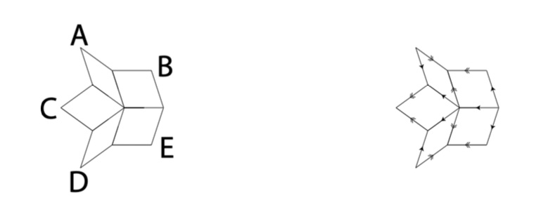
We still have to show that this gives a legal Rhombic tiling, that is, that the gluing restrictions of Penrose’s rhombs are satisfied.

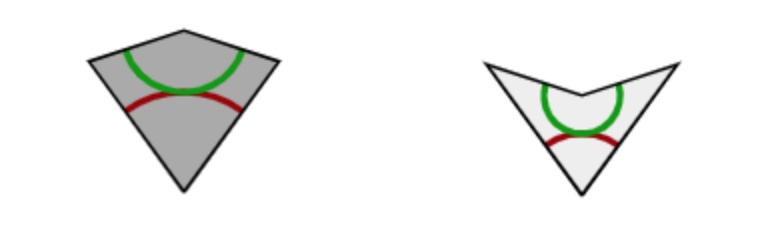
We do this by orienting and colouring the edges of the thin and thick rhombus towards the vertex defined by the semi-circles on the rhombus-pieces. Edges connecting a point of index $3$ to a point of index $2$ are coloured red, edges connecting a point of index $1$ to a point of index $2$, or connecting a point of index $3$ to one of index $4$ are coloured blue.

We orient green edges pointing from index $2$ to index $1$, or from index $3$ to index $4$. As this orientation depends only on the index-values of the vertices, two rhombs sharing a common green edge also have the same orientation on that edge.

On each individual rhomb, knowing the green edges and their orientation forced the red edges and their orientation, but we still have to show that if two rhombs share a common red edge, this edge has the same orientation on both (note in the picture above that a red edge can both flow from $2$ to $3$ as well as from $3$ to $2$).

From the gluing conditions of Penrose’s rhombs we see that if $PQ$ be a red edge, in common to two rhombs, and these rhombs have angle $\alpha$ resp. $\beta$ in $P$, then $\alpha$ and $\beta$ must be both less that $90^o$ or both bigger than $90^o$. We translate this in terms of the pentragrid.

The two rhombs correspond to two intersection points $A$ and $B$, and we may assume that they both lie on a line $l$ of family $0$ of parallel lines (other cases are treated similarly by cyclic permutation), and that $A$ is an intersection with a family $p$-line and $B$ with a family $q$-line, with $p,q \in \{ 1,2,3,4 \}$. The interval $AB$ crosses the unique edge common to the two rhombs determined by $A$ and $B$, and we call the interval $AB$ red if $\sum_j K_j(\vec{x})$ is $2$ on one side of $AB$ and $3$ on the other side. The claim about the angles $\alpha$ and $\beta$ above now translates to: if $AB$ is red, then $p+q$ is odd (in the picture above $p=1$ and $q=2$).

By a transformation we may assume that $\gamma_0=0$ and that $l$ is the $Y$-axis. For every $y \in \mathbb{R}$ we then get
\[
\begin{cases}
K_1(0,y) = \lceil y .sin(2 \pi/5) + \gamma_1 \rceil \\
K_2(0,y) = \lceil y .sin(4 \pi/5) + \gamma_2 \rceil \\
K_3(0,y) = \lceil -y .sin(4 \pi/5) + \gamma_3 \rceil \\
K_4(0,y) = \lceil -y .sin(2 \pi/5) + \gamma_4 \rceil
\end{cases}
\]
and $\gamma_1+\gamma_4$ and $\gamma_2+\gamma_3$ are not integers (otherwise the pentagrid is not regular). If $y$ runs from $-\infty$ to $+\infty$ we find that
\[
K_1(0,y)+K_4(0,y) – \lceil \gamma_1 + \gamma_4 \rceil = \begin{cases} 0 \\ 1 \end{cases} \]
with jumps from $0$ to $1$ at places where $(\lceil \gamma_1 + \gamma_4 \rceil – \gamma_1)/sin(2 \pi/5) \in \mathbb{Z}$ and from $1$ to $0$ when $\gamma_4/sin(2 \pi/5) \in \mathbb{Z}$. (A similar result holds replacing $K_1,K_4,\gamma_1,\gamma_4,sin(2 \pi/5)$ by $K_2,K_3,\gamma_2,\gamma_3,sin(4 \pi/5)$.

Because the points on $l$ intersecting with $1$-family and $4$-family gridlines alternate (and similarly for $2$- and $3$-family gridlines) we know already that $p \not= q$. If we assume that $p+q$ is even, we have two possibilities, either $\{p,g \}=\{ 1,3 \}$ or $\{ 2,4 \}$. As $\gamma_0=0$ we have $\gamma_1+\gamma_2+\gamma_3+\gamma_4=0$ and therefore
\[
\lceil \gamma_1 + \gamma_4 \rceil + \lceil \gamma_2+\gamma_3 \rceil = 1 \]
It then follows that $K_1(0,y)+K_2(0,y)+K_3(0,y)+K_4(0,y) = 1$ or $3$ between the points $A$ and $B$. Therefore $K_0(y,0) + \dots + K_4(0,y)$ is either $1$ on the left side and $2$ on the right side, or is $3$ on the left side and $4$ on the right side, so $AB$ must be green, a contradiction. Therefore, $p+q$ is odd, and the orientation of the red edge in both rhombs is the same. Done!

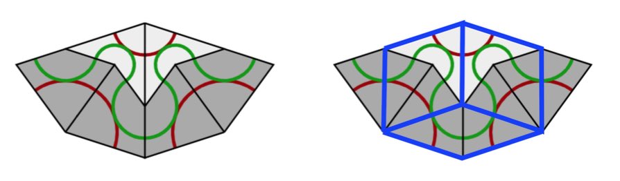
An alternative way to see this correspondence between regular pentagrids and Rhombic tilings as as follows. To every intersection of two gridlines we assign a rhombus, a thin one if they meet at an acute angle of $36^o$ and a thich one if this angle is $72^o$, with the long diagonal dissecting the obtuse angle.

Do this for all intersections, surrounding a given mesh.

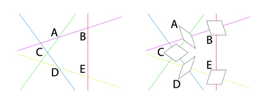
Attach the rhombs by translating them towards the mesh, and finally draw the colours of the edges.

Another time, we will connect this to the cut-and-project method, using the representation theory of $D_5$.

Penrose’s aperiodic tilings

Published March 9, 2021 by lievenlb

Around 1975 Sir Roger Penrose discovered his aperiodic P2 tilings of the plane, using only two puzzle pieces: Kites (K) and Darts (D)

The inner angles of these pieces are all multiples of $36^o = \tfrac{180^o}{5}$, the short edges have length $1$, and the long edges have length $\tau = \tfrac{1+\sqrt{5}}{2}$, the golden ratio. These pieces must be joined together so that the colours match up (if we do not use this rule it is easy to get periodic tilings with these two pieces).

There is plenty of excellent online material available:

The two original Martin Gardner Scientific American articles on Penrose tiles have been made available by the MAA, and were reprinted in “Penrose Tiles to Trapdoor Ciphers”. They contain most of Conway’s early discoveries about these tilings, but without proofs.
A JavaScript application by Kevin Bertman to play around with these tilings. You can deflate and inflate tilings, find forced tiles and much more. Beneath the app-window there’s a detailed explanation of all the basics, including inflation and deflation of the P2-tiles, the seven types of local vertex configurations (naming by Conway, of course),

proofs of aperiodicity (similar to the one for Conway’s musical sequences), that every tile lies within an ace (similar to the LSL-subword in musical sequences) with application to local isomorphism (again similar to the $1$-dimensional case).
Course notes of an Oxford masterclass in geometry Lectures on Penrose tilings by Alexander Ritter, again with proofs of all of the above and a discussion about the Cartwheel tilings (similar to that in the post on musical sequences), giving an algorithm to decide whether or not a partial tiling can be extended to the entire plane, or not.

There’s no point copying this material here. Rather, I’d like to use some time in this GoV series of posts to talk about de Bruijn’s pentagrid results. For this reason, I now need to make the connection with Penrose’s ‘other’ tilings, the P3 tiles of ‘thin’ and ‘thick’ rhombi (sometimes called ‘skinny’ and ‘fat’ rhombi).

Every Penrose P2-tiling can be turned into a P3-rhombic tiling, and conversely.

From kites and darts to rhombi: divide every kite in two halves along its line of reflection. Then combine darts and half-kites into rhombi where a fat rhombus consists of a dart and two half-kites, joined at a long edge, and a skinny rhombus is made of two half-kites, joined at a short edge. This can always be done preserving the gluing conditions. It suffices to verify this for the deflated kite and dart (on the left below) and we see that the matching colour-conditions are those of the rhombi.

From rhombi to kites and darts: divide every fat rhombus into a dart (placed at the red acute angle) and two half-kites, joined at a long edge, and divide every skinny rhombus into two half-kites along its short diagonal.

All results holding for Kites and Darts tilings have therefore their versions for Rhombic tilings. For example, we have rhombic deflation and inflation rules

A Rhombic tiling can be seen as an intermediate step in the inflation process of a Penrose tiling $P$. Start by dividing all kites in two halves along their long diagonal and all darts in two halves along their short diagonal (the purple lines below).

If we consider all original black lines together with the new purple ones, we get a tiling of the plane by triangles and we call this the $A$-tiling. There are two triangles, s small triangle $S_A$ (the whiter ones, with two small edges ofd length $1$ and one edge of length $\tau$) and a large triangle $L_A$ (the greyer ones, with two edges of length $\tau$ and one edge of length $1$).

Next, we remove the black lines joining an $S_A$-triangle with an $L_A$-triangle, and get another tiling with triangles, the $B$-tiling, with two pieces, a large triangle $L_B$ with two sides of length $\tau$ and one side of length $1+\tau$ (the white ones) (the union of an $L_A$ and a $S_A$), and a small triangle $S_B$ which has the same form as $L_A$ (the greyer ones). If we now join two white triangles $L_B$ along their common longer edge, and two greyer triangles $S_B$ along their common smaller edge, we obtain the Rhombic tiling $R$ corresponding to $P$.

We can repeat this process starting with the Rhombic tiling $R$. We divide all fat rhombi in two along their long diagonals, and the skinny rhombi in two along their short diagonals (the purple lines). We obtain a tiling of the plane by triangles, which is of course just the $B$-tiling above.

Remove the edge joining a small $S_B$ with a large $L_B$ triangle, then we get a new tiling by triangles, the $\tau A$-tiling consisting of large triangles $L_{\tau A}$ (the white ones) with two long edges of length $1+\tau$ and one short edge of length $\tau$ (note that $L_{\tau A}$ is $\tau$ times the triangle $L_A$), and a smaller one $S_{\tau A}$ (the grey ones) having two short edges of length $\tau$ and one long edge of length $1+\tau$ (again $S_{\tau A}$ is $\tau$ times the triangle $S_A$). If we join two $L_{\tau A}$-triangles sharing a common long edge we obtain a Kite ($\tau$-times larger than the original Kite) and if we joint two $S_{\tau A}$-triangles along their common small edge we get a Dart ($\tau$ times larger than the original Dart). The Penrose tiling we obtain is the inflation $inf(P)$ of the original $P$.

If we repeat the whole procedure starting from $inf(P)$ instead of $P$ we get, in turn, triangle tilings of the plane, subsequently the $\tau B$-tiling, the $\tau^2 A$-tiling, the $\tau^2 B$-tiling and so on, the triangles in a $\tau^n A$-tiling being of size $\tau^2$-times those of the $A$-tiling, and those in the $\tau^n B$-tiling $\tau^n$-times as large as those of the $B$-tiling.

The upshot of this is that we can associate to a Penrose tiling $P$ of the plane a sequence of $0$’s and $1$’s. Starting from $P$ we have an infinite sequence of associated triangle tilings
\[
A,~B,~\tau A,~\tau B,~\tau^2 A, \dots,~\tau^n A,~\tau^n B,~\tau^{n+1} A, \dots \]
with larger and larger triangle tiles. Let $p$ be a point of the plane lying in the interior of an $A$-tile, then we define its index sequence
\[
i(P,p) = (x_0,x_1,x_2,\dots ) \quad x_{2n} = \begin{cases} 0~\text{if $p \in L_{\tau^n A}$} \\ 1~\text{if $p \in S_{\tau^n A}$} \end{cases}~ x_{2n+1} = \begin{cases} 0~\text{if $p \in L_{\tau^n B}$} \\ 1~\text{if $p \in S_{\tau^n B}$} \end{cases} \]
That is, $x_0=1$ if $p$ lies in a small triangle of the $A$-tiling and $x_0=1$ if it lies in a large triangle, $x_1=1$ if $p$ lies in a small triangle of the $B$-tiling and is $0$ if it lies in a large $B$-triangle, and so on.

The beauty of this is that every infinite sequence $(x_0,x_1,x_2,\dots )$ whose terms are $0$ or $1$, and in which no two consecutive terms are equal to $1$, is the index sequence $i(P,p)$ of some Penrose tiling $P$ in some point $p$ of the plane.

From the construction of the sequence of triangle-tilings it follows that a small triangle is part of a large triangle in the next tiling. For this reason an index sequence can never have two consecutive ones. An index sequence gives explicit instructions as to how the Penrose tiling is constructed. In each step add a large or small triangle as to fit the sequence, together with the matching triangle (the other half of a Penrose or Rhombic tile). Next, look at the patches $P_i$ of Kites and Darts (in the $\tau^i A$ tiling), for $i=0,1,\dots$, then $P_{i-k}$ is contained in the $k$-times inflated $P_i$, $i^k(P_i)$ (without rescaling), for each $i$ and all $1 \leq k \leq i$. But then, we have a concentric series of patches
\[
P_0 \subset i(P_1) \subset i^2(P_2) \subset \dots \]
filling the entire plane.

The index sequence depends on the choice of point $p$ in the plane. If $p’$ is another point, then as the triangle tiles increase is size at each step, $p$ and $p’$ will lie in the same triangle-tile at some stage, and after that moment their index sequences will be the same.

As a result, there exists an uncountable infinity of distinct Penrose tilings of the plane.

From the discussions we see that a Penrose tiling is determined by the index-sequence in any point in the plane $(x_0,x_1,\dots )$ consisting of $0$’s and $1$’s having no two consecutive $1$’s, and that another such sequence $(x’_0,x’_1,\dots )$ determines the same Penrose tilings if $x_n=x’_n$ for all $n \geq N$ for some number $N$. That is, the Penrose tiling is determined by the the equivalence class of such sequences, and it is easy to see that there are uncountably many such equivalence classes.

If you want to play a bit with Penrose tiles, you can order the P2 tiles or the P3 tiles from
Cherry Arbor Design.

Conway’s musical sequences

Published March 2, 2021 by lievenlb

Before we’ll come to applications of quasicrystals to viruses it is perhaps useful to illustrate essential topics such as deflation, inflation, aperiodicity, local isomorphism and the cut-and project method in the simplest of cases, that of $1$-dimensional tilings.

We want to tile the line $\mathbb{R}^1$ with two kinds of tiles, short ($S$) and ($L$) long intervals, differing by a golden ratio factor $\tau=\tfrac{1}{2}(1+\sqrt{5}) \approx 1.618$.

Clearly, no two tiles may overlap and we impose a gluing restriction: there can be no two consecutive $S$-intervals in the tiling, and no three consecutive $L$-intervals.

The code of a tiling is a doubly infinite word in $S$ and $L$ such that there are no two consecutive $S$’s nor three consecutive $L$’s. For example
\[
\sigma = \dots LSLLSLS\underline{L}LSLLSL \dots \]
We underline one tile to distinguish the sequence from shifts of it.

Conway’s musical sequences will be special codes (or tilings), allowing for the inverse operations of inflation and deflation, terms coined by John Conway in relation to Penrose tilings. The musical sequences are important to understand Conway’s worms (sometimes called “wormholes”) which are strings of Long and Short bow ties in a Penrose tiling, and to measure the distances between Amman bars. In fact, many of the properties of Penrose tilings and $3$-dimensional quasicrystals (for example, local isomorphism) have their counterparts for tilings having a musical sequence as code.

Conway’s investigations of Penrose tiles held up work on the ATLAS-project and caused some problems at home:

“In pursuing his investigations, he unsurped some of his wife Eileen’s territory, covering the dining table with an infinite nuisance of tiles. He cut them out himself, causing his right hand to hurt with cramps for days. To Eileen’s dismay, he studied the dining table mosaic for a year, relegating family meals to the kitchen and prohibiting dinner parties.”

From “Genius at Play – The curious mind of John Horton Conway” by Siobhan Roberts

Let’s investigate inflation and deflation of these tilings.

The point of the golden factor $\tau$ is to allow for deflation. That is, we can replace a tiling by another one with tiles $S$ and $L$ both a factor $\tfrac{1}{\tau}=\tau-1 \approx 0.618$ smaller than the original tiles. If the original $S$-tile has length $a$ (and the $L$-tile length $\tau a$), then the new tile $S$ wil have length $\tfrac{1}{\tau}a$ and the new $L$-tile length $a$.
We do this by replacing each old $S$-tile by a new $L$-tile, and to break up any old $L$-tile in a new $L$ and new $S$-tile, as $\tau a = a + \tfrac{1}{\tau}a$ (note that $\tau^2=\tau+1$)

To get the code of the deflated tiling we replace each letter $S$ by a letter $L$ and each $L$ by $LS$. The underlined letter will be the first letter of the deflated underlined letter in the original sequence. The deflated sequence of the one above is
\[
def(\sigma) = \dots LSLLSLSLLSL\underline{L}SLSLLSLSLLS \dots \]
and it is easy to see that the deflated tiling satisfies again the gluing condition.

Certain of these tilings (not all!) allow for an inverse to deflation, called inflation, increasing the size of the tiles by a factor $\tau$.

Starting from a tiling we divide each $L$-tile in half and these mid-points will be end-points of the tiles in the new tiling, erasing all endpoints of the original one. The inflated tiling will have two sorts of tiles, a new short one $S$ of length $\tau a$ obtained from the end-half of an original $L$-tile, followed b the start-half of an original $L$-tile, and a new long tile $L$ of length $\tau^2 a = (\tau+1) a$, made of the end-half of an original $L$, followed by an original $S$, followed by the start-half of an original $L$.

We get the code of the inflated tiling by replacing first each $L$ by $ll$ and subsequently replace each word $lSl$ by a letter $L$ and each $ll$ by $S$. An example,
\[
\sigma = \dots LSLLSLSLLSL\underline{L}SLSLLSLSLLS \dots \\
\dots llSllllSllSllllSlll\underline{l}SllSllllSllSllllS \dots \\
inf(\sigma) = \dots (l)LSLLSLS\underline{L}LSLLS(lS) \dots \]

But, the inflated tiling may no longer satisfy the gluing condition. An example
\[
\dots LSLSLSL \dots \mapsto \dots llSllSllSll \dots \mapsto \dots (l)LLL(l) \dots \]

A Conway musical sequence is the code of a tiling $\sigma$ such that all its consecutive inflations $inf^n(\sigma)$ satisfy the gluing condition. For the corresponding Conway tiling $\sigma$ we have that
\[
def(inf(\sigma))=\sigma=inf(def(\sigma)) \]

Let’s construct at least two such Conway tilings (later we’ll see that there are uncountably many). Take $C_n=def^n(LS\underline{L})$ and write it in a special form to highlight symmetries.
\begin{eqnarray*}
C_0 =& (L.S)\underline{L} \\
C_1 =& L(S.L)\underline{L}S \\
C_2 =& LSL(L.S)\underline{L}SL \\
C_3 =& LSLLSL(S.L)\underline{L}SLLS \\
C_4 =& LSLLSLSLLSL(L.S)\underline{L}SLLSLSL
\end{eqnarray*}

The even terms have middle-part $(L.S)$ and the odd ones $(S.L)$. The remaing left and right parts are each others reflexion (or part of it). This is easily seen by induction as are the inclusions
\[
C_0 \subset C_2 \subset C_4 \subset \dots \subset C_{even} \quad \text{and} \quad C_1 \subset C_3 \subset C_5 \subset \dots \subset C_{odd} \]

$C_{even}$ and $C_{odd}$ are special Conway musical sequences, called the middle $C$-sequences, and are each others inflation and deflation. If you are familiar with Penrose tilings, these are the $1$-dimensional counterparts of the cartwheel Penrose tiling (here with the $10$ Conway worms emanating from the center, and with the borders of the first few cartwheels drawn).

A direct consequence of inflation on Conway’s musical sequences is that the corresponding tiling is aperiodic, that is, it has no translation symmetry.

For, inflation only depends on the local configuration of tiles, so if translation by $R$ is a symmetry of a musical sequence $\sigma$ then it is also a symmetry of $inf(\sigma)$, and so also of $inf^n(\sigma)$. But for large $n$ we will have that $R < \tau^n a$ (with $a$ the size of the tiles in $\sigma$). But then a tile in $inf^n(\sigma)$ and its translation by $R$ must overlap which is impossible if $+R$ is a translation symmetry of $inf^n(\sigma)$. Done!

Returning to the middle C-sequences, what was the point of starting with $C_0 = LSL$? Well, it follows directly from the gluing restrictions that any letter in a musical sequence is part of a subword $LSL$ of $\sigma$. But then, every finite subword $W$ of $\sigma$ is also a subword of $C_{2n}$ for some large $n$.

For, let $d$ be the length of the interval corresponding to $W$ and choose $n$ such that $d > \tau^{2n} a$ then the interval of the line corresponding to $W$ is contained in a single tile in $inf^{2n}(\sigma)$ and this tile belongs to a subword $LSL$ of $inf^{2n}(\sigma)$. But then $W$ will be a subword of the $2n$-th deflation of that interval $LSL \subset inf^{2n}(\sigma)$, which is $C_{2n}$.

Or, as Conway would phrase it with respect to Penrose tilings (quote again from Siobhan Roberts’ book)

“Every points is in the cartwheel somewhere. If you jab your finger anywhere, on any point anywhere on teh pattern, you are part of a cartwheel. The whole ting is overlapping cartwheels.”

An immediate consequence is the local isomorphism theorem: Every subword of a musical sequence $\sigma$ appears infinitely many times as subword of any other musical sequence. That is, one cannot distinguish two tilings of the line with musical sequence codes from each other by looking at finite intervals!

The argument is similar to the one above. The finite interval corresponding to the subword lies in a unique tile of $inf^n(\sigma)$ for $n$ large enough. Now, take another musical sequence $\mu$ and consider any of the infinitely many tiles of the same type in $inf^n(\mu)$, then $def^n$ of such a tile will contain the subword in $\phi$.

Another time, we’ll see that musical sequences can be produced by the ‘cut-and-project’-method (what I called the ‘windows’-method before).
This time we will project parts of the standard $2$-dimensional lattice $\mathbb{Z}^2$ onto the line, which is a lot easier to visualise than de Bruijn’s projection from $\mathbb{R}^5$ to produce Penrose tilings or the projection from six dimensional space to harvest quasicrystals.