I really like Matilde Marcolli’s idea to use some of Jackson Pollock’s paintings as metaphors for noncommutative spaces. In her talk she used this painting
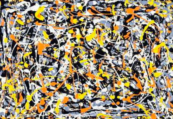
and refered to it (as did I in my post) as : Jackson Pollock “Untitled N.3”. Before someone writes a post ‘The Pollock noncommutative space hoax’ (similar to my own post) let me point out that I am well aware of the controversy surrounding this painting.
 This painting is among 32 works recently discovered and initially attributed to Pollock.
In fact, I’ve already told part of the story in Doodles worth millions (or not)? (thanks to PD1). The story involves the people on the right : from left to right, Jackson Pollock, his wife Lee Krasner, Mercedes Matter and her son Alex Matter.
Alex Matter, whose father, Herbert, and mother, Mercedes, were artists and friends of Jackson Pollock, discovered after his mother died a group of small drip paintings in a storage locker in Wainscott, N.Y. which he believed to be authentic Pollocks.
Read the post mentioned above if you want to know how mathematics screwed up his plan, or much better, reed the article Anatomy of the Jackson Pollock controversy by Stephen Litt.
So, perhaps the painting above was not the smartest choice, but we could take any other genuine Pollock ‘drip-painting’, a technique he taught himself towards the end of 1946 to make an image by splashing, pouring, sloshing colors onto the canvas. Typically, such a painting consists of blops of paint, connected via thin drip-lines.
What does this have to do with noncommutative geometry? Well, consider the blops as ‘points’. In commutative geometry, distinct points cannot share tangent information ((technically : a commutative semi-local ring splits as the direct sum of local rings and this does no longer hold for a noncommutative semi-local ring)). In the noncommutative world though, they can!, or if you want to phrase it like this, noncommutative points ‘can talk to each other’. And, that’s what we cherish in those drip-lines.
But then, if two points share common tangent informations, they must be awfully close to each other… so one might imagine these Pollock-lines to be strings holding these points together. Hence, it would make more sense to consider the ‘Pollock-quotient-painting’, that is, the space one gets after dividing out the relation ‘connected by drip-lines’ ((my guess is that Matilde thinks of the lines as the action of a group on the points giving a topological horrible quotient space, and thats precisely where noncommutative geometry shines)).
For this reason, my own mental picture of a genuinely noncommutative space ((that is, the variety corresponding to a huge noncommutative algebra such as free algebras, group algebras of arithmetic groups or fundamental groups)) looks more like the picture below
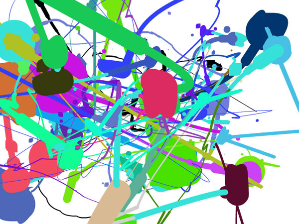
The colored blops you see are really sets of points which you might view as, say, a FacebookGroup ((technically, think of them as the connected components of isomorphism classes of finite dimensional simple representations of your favorite noncommutative algebra)). Some chatter may occur between two distinct FacebookGroups, the more chatter the thicker the connection depicted ((technically, the size of the connection is the dimension of the ext-group between generic simples in the components)). Now, there are some tiny isolated spots (say blue ones in the upper right-hand quadrant). These should really be looked at as remote clusters of noncommutative points (sharing no (tangent) information whatsoever with the blops in the foregound). If we would zoom into them beyond the Planck scale (if I’m allowed to say a bollock-word in a Pollock-post) they might reveal again a whole universe similar to the interconnected blops upfront.
The picture was produced using the fabulous Pollock engine. Just use your mouse to draw and click to change colors in order to produce your very own noncommutative space!
For the mathematicians still around, this may sound like a lot of Pollock-bollocks but can be made precise. See my note Noncommutative geometry and dual coalgebras for a very terse reading. Now that coalgebras are gaining popularity, I really should write a more readable account of it, including some fanshi-wanshi examples…
4 Comments
 Both posts were influential to