Tag: modular

looking for the moonshine picture

Published May 11, 2009 by lievenlb

We have seen that Conway’s big picture helps us to determine all arithmetic subgroups of $PSL_2(\mathbb{R}) $ commensurable with the modular group $PSL_2(\mathbb{Z}) $, including all groups of monstrous moonshine.

As there are exactly 171 such moonshine groups, they are determined by a finite subgraph of Conway’s picture and we call the minimal such subgraph the moonshine picture. Clearly, we would like to determine its structure.

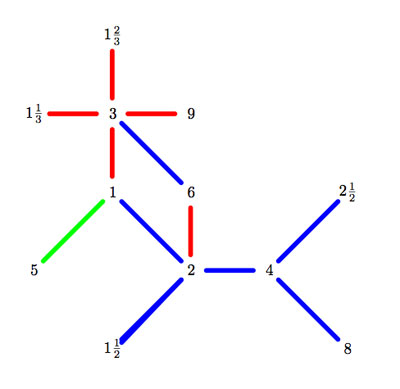
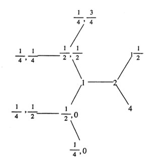
On the left a depiction of a very small part of it. It is the minimal subgraph of Conway’s picture needed to describe the 9 moonshine groups appearing in Duncan’s realization of McKay’s E(8)-observation. Here, only three primes are relevant : 2 (blue lines), 3 (reds) and 5 (green). All lattices are number-like (recall that $M \frac{g}{h} $ stands for the lattice $\langle M e_1 + \frac{g}{h} e_2, e_2 \rangle $).

We observe that a large part of this mini-moonshine picture consists of the three p-tree subgraphs (the blue, red and green tree starting at the 1-lattice $1 = \langle e_1,e_2 \rangle $. Whereas Conway’s big picture is the product over all p-trees with p running over all prime numbers, we observe that the mini-moonshine picture is a very small subgraph of the product of these three subtrees. In fact, there is just one 2-cell (the square 1,2,6,3).

Hence, it seems like a good idea to start our investigation of the full moonshine picture with the determination of the p-subtrees contained in it, and subsequently, worry about higher dimensional cells constructed from them. Surely it will be no major surprise that the prime numbers p that appear in the moonshine picture are exactly the prime divisors of the order of the monster group, that is p=2,3,5,7,11,13,17,19,23,29,31,41,47,59 or 71. Before we can try to determine these 15 p-trees, we need to know more about the 171 moonshine groups.

Recall that the proper way to view the modular subgroup $\Gamma_0(N) $ is as the subgroup fixing the two lattices $L_1 $ and $L_N $, whence we will write $\Gamma_0(N)=\Gamma_0(N|1) $, and, by extension we will denote with $\Gamma_0(X|Y) $ the subgroup fixing the two lattices $L_X $ and $L_Y $.

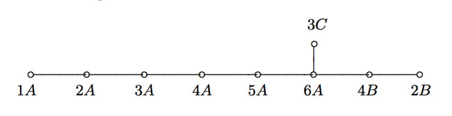
As $\Gamma_0(N) $ fixes $L_1 $ and $L_N $ it also fixes all lattices in the (N|1)-thread, that is all lattices occurring in a shortest path from $L_1 $ to $L_N $ (on the left a picture of the (200|1)-thread).

If $N=p_1^{a_1} p_2^{a_2} \ldots p_k^{a_k} $, then the (N|1)-thread has $2^k $ involutions as symmetries, called the Atkin-Lehner involutions. For every exact divisor $e || N $ (that is, $e|N $ and $gcd(e,\frac{N}{e})=1 $ we have an involution $W_e $ which acts by sending each point in the thread-cell corresponding to the prime divisors of $e $ to its antipodal cell-point and acts as the identity on the other prime-axes. For example, in the (200|1)-thread on the left, $W_8 $ is the left-right reflexion, $W_{25} $ the top-bottom reflexion and $W_{200} $ the antipodal reflexion. The set of all exact divisors of N becomes the group $~(\mathbb{Z}/2\mathbb{Z})^k $ under the operation $e \ast f = \frac{e \times f}{gcd(e,f)^2} $.

Most of the moonshine groups are of the form $\Gamma_0(n|h)+e,f,g,… $ for some $N=h.n $ such that $h | 24 $ and $h^2 | N $. The group $\Gamma_0(n|h) $ is then conjugate to the modular subgroup $\Gamma_0(\frac{n}{h}) $ by the element $\begin{bmatrix} h & 0 \ 0 & 1 \end{bmatrix} $. With $\Gamma_0(n|h)+e,f,g,… $ we mean that the group $\Gamma_0(n|h) $ is extended with the involutions $W_e,W_f,W_g,… $. If we simply add all Atkin-Lehner involutions we write $\Gamma_0(n|h)+ $ for the resulting group.

Finally, whenever $h \not= 1 $ there is a subgroup $\Gamma_0(n||h)+e,f,g,… $ which is the kernel of a character $\lambda $ being trivial on $\Gamma_0(N) $ and on all involutions $W_e $ for which every prime dividing $e $ also divides $\frac{n}{h} $, evaluating to $e^{\frac{2\pi i}{h}} $ on all cosets containing $\begin{bmatrix} 1 & \frac{1}{h} \ 0 & 1 \end{bmatrix} $ and to $e^{\pm \frac{2 \pi i }{h}} $ for cosets containing $\begin{bmatrix} 1 & 0 \ n & 0 \end{bmatrix} $ (with a + sign if $\begin{bmatrix} 0 & -1 \ N & 0 \end{bmatrix} $ is present and a – sign otherwise). Btw. it is not evident at all that this is a character, but hard work shows it is!

Clearly there are heavy restrictions on the numbers that actually occur in moonshine. In the paper On the discrete groups of moonshine, John Conway, John McKay and Abdellah Sebbar characterized the 171 arithmetic subgroups of $PSL_2(\mathbb{R}) $ occuring in monstrous moonshine as those of the form $G = \Gamma_0(n || h)+e,f,g,… $ which are

(a) of genus zero, meaning that the quotient of the upper-half plane by the action of $G \subset PSL_2(\mathbb{R}) $ by Moebius-transformations gives a Riemann surface of genus zero,
(b) the quotient group $G/\Gamma_0(nh) $ is a group of exponent 2 (generated by some Atkin-Lehner involutions), and
(c) every cusp can be mapped to $\infty $ by an element of $PSL_2(\mathbb{R}) $ which conjugates the group to one containing $\Gamma_0(nh) $.

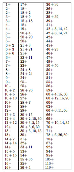
Now, if $\Gamma_0(n || h)+e,f,g,… $ is of genus zero, so is the larger group $\Gamma_0(n | h)+e,f,g,… $, which in turn, is conjugated to the group $\Gamma_0(\frac{n}{h})+e,f,g,… $. Therefore, we need a list of all groups of the form $\Gamma_0(\frac{n}{h})+e,f,g,… $ which are of genus zero. There are exactly 123 of them, listed on the right.

How does this help to determine the structure of the p-subtree of the moonshine picture for the fifteen monster-primes p? Look for the largest p-power $p^k $ such that $p^k+e,f,g… $ appears in the list. That is for p=2,3,5,7,11,13,17,19,23,29,31,41,47,59,71 these powers are resp. 5,3,2,2,1,1,1,1,1,1,1,1,1,1,1. Next, look for the largest p-power $p^l $ dividing 24 (that is, 3 for p=2, 1 for p=3 and 0 for all other primes). Then, these relevant moonshine groups contain the modular subgroup $\Gamma_0(p^{k+2l}) $ and are contained in its normalizer in $PSL_2(\mathbb{R}) $ which by the Atkin-Lehner theorem is precisely the group $\Gamma_0(p^{k+l}|p^l)+ $.

Right, now the lattices fixed by $\Gamma_0(p^{k+2l}) $ (and permuted by its normalizer), that is the lattices in our p-subtree, are those that form the $~(p^{k+2l}|1) $-snake in Conway-speak. That is, the lattices whose hyper-distance to the $~(p^{k+l}|p^l) $-thread divides 24. So for all primes larger than 2 or 3, the p-tree is just the $~(p^l|1) $-thread.

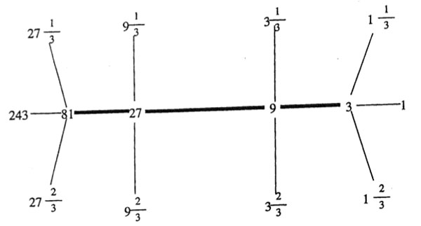
For p=3 the 3-tree is the (243|1)-snake having the (81|3)-thread as its spine. It contains the following lattices, all of which are number-like.

Depicting the 2-tree, which is the (2048|1)-snake may take a bit longer… Perhaps someone should spend some time figuring out which cells of the product of these fifteen trees make up the moonshine picture!

4 Comments

Conway’s big picture

Published May 2, 2009 by lievenlb

Conway and Norton showed that there are exactly 171 moonshine functions and associated two arithmetic subgroups to them. We want a tool to describe these and here’s where Conway’s big picture comes in very handy. All moonshine groups are arithmetic groups, that is, they are commensurable with the modular group. Conway’s idea is to view several of these groups as point- or set-wise stabilizer subgroups of finite sets of (projective) commensurable 2-dimensional lattices.

Expanding (and partially explaining) the original moonshine observation of McKay and Thompson, John Conway and Simon Norton formulated monstrous moonshine :

To every cyclic subgroup $\langle m \rangle $ of the Monster $\mathbb{M} $ is associated a function

$f_m(\tau)=\frac{1}{q}+a_1q+a_2q^2+\ldots $ with $q=e^{2 \pi i \tau} $ and all coefficients $a_i \in \mathbb{Z} $ are characters at $m $ of a representation of $\mathbb{M} $. These representations are the homogeneous components of the so called Moonshine module.

Each $f_m $ is a principal modulus for a certain genus zero congruence group commensurable with the modular group $\Gamma = PSL_2(\mathbb{Z}) $. These groups are called the moonshine groups.

Conway and Norton showed that there are exactly 171 different functions $f_m $ and associated two arithmetic subgroups $F(m) \subset E(m) \subset PSL_2(\mathbb{R}) $ to them (in most cases, but not all, these two groups coincide).

Whereas there is an extensive literature on subgroups of the modular group (see for instance the series of posts starting here), most moonshine groups are not contained in the modular group. So, we need a tool to describe them and here’s where Conway’s big picture comes in very handy.

All moonshine groups are arithmetic groups, that is, they are subgroups $G $ of $PSL_2(\mathbb{R}) $ which are commensurable with the modular group $\Gamma = PSL_2(\mathbb{Z}) $ meaning that the intersection $G \cap \Gamma $ is of finite index in both $G $ and in $\Gamma $. Conway’s idea is to view several of these groups as point- or set-wise stabilizer subgroups of finite sets of (projective) commensurable 2-dimensional lattices.

Start with a fixed two dimensional lattice $L_1 = \mathbb{Z} e_1 + \mathbb{Z} e_2 = \langle e_1,e_2 \rangle $ and we want to name all lattices of the form $L = \langle v_1= a e_1+ b e_2, v_2 = c e_1 + d e_2 \rangle $ that are commensurable to $L_1 $. Again this means that the intersection $L \cap L_1 $ is of finite index in both lattices. From this it follows immediately that all coefficients $a,b,c,d $ are rational numbers.

It simplifies matters enormously if we do not look at lattices individually but rather at projective equivalence classes, that is $~L=\langle v_1, v_2 \rangle \sim L’ = \langle v’_1,v’_2 \rangle $ if there is a rational number $\lambda \in \mathbb{Q} $ such that $~\lambda v_1 = v’_1, \lambda v_2=v’_2 $. Further, we are of course allowed to choose a different ‘basis’ for our lattices, that is, $~L = \langle v_1,v_2 \rangle = \langle w_1,w_2 \rangle $ whenever $~(w_1,w_2) = (v_1,v_2).\gamma $ for some $\gamma \in PSL_2(\mathbb{Z}) $.
Using both operations we can get any lattice in a specific form. For example,

$\langle \frac{1}{2}e_1+3e_2,e_1-\frac{1}{3}e_2 \overset{(1)}{=} \langle 3 e_1+18e_2,6e_1-2e_2 \rangle \overset{(2)}{=} \langle 3 e_1+18 e_2,38 e_2 \rangle \overset{(3)}{=} \langle \frac{3}{38}e_1+\frac{9}{19}e_2,e_2 \rangle $

Here, identities (1) and (3) follow from projective equivalence and identity (2) from a base-change. In general, any lattice $L $ commensurable to the standard lattice $L_1 $ can be rewritten uniquely as $L = \langle Me_1 + \frac{g}{h} e_2,e_2 \rangle $ where $M $ a positive rational number and with $0 \leq \frac{g}{h} < 1 $.

Another major feature is that one can define a symmetric hyper-distance between (equivalence classes of) such lattices. Take $L=\langle Me_1 + \frac{g}{h} e_2,e_2 \rangle $ and $L’=\langle N e_1 + \frac{i}{j} e_2,e_2 \rangle $ and consider the matrix

$D_{LL’} = \begin{bmatrix} M & \frac{g}{h} \\ 0 & 1 \end{bmatrix} \begin{bmatrix} N & \frac{i}{j} \\ 0 & 1 \end{bmatrix}^{-1} $ and let $\alpha $ be the smallest positive rational number such that all entries of the matrix $\alpha.D_{LL’} $ are integers, then

$\delta(L,L’) = det(\alpha.D_{LL’}) \in \mathbb{N} $ defines a symmetric hyperdistance which depends only of the equivalence classes of lattices (hyperdistance because the log of it behaves like an ordinary distance).

Conway’s big picture is the graph obtained by taking as its vertices the equivalence classes of lattices commensurable with $L_1 $ and with edges connecting any two lattices separated by a prime number hyperdistance. Here’s part of the 2-picture, that is, only depicting the edges of hyperdistance 2.

The 2-picture is an infinite 3-valent tree as there are precisely 3 classes of lattices at hyperdistance 2 from any lattice $L = \langle v_1,v_2 \rangle $ namely (the equivalence classes of) $\langle \frac{1}{2}v_1,v_2 \rangle~,~\langle v_1, \frac{1}{2} v_2 \rangle $ and $\langle \frac{1}{2}(v_1+v_2),v_2 \rangle $.

Similarly, for any prime hyperdistance p, the p-picture is an infinite p+1-valent tree and the big picture is the product over all these prime trees. That is, two lattices at square-free hyperdistance $N=p_1p_2\ldots p_k $ are two corners of a k-cell in the big picture!
(Astute readers of this blog (if such people exist…) may observe that Conway’s big picture did already appear here prominently, though in disguise. More on this another time).

The big picture presents a simple way to look at arithmetic groups and makes many facts about them visually immediate. For example, the point-stabilizer subgroup of $L_1 $ clearly is the modular group $PSL_2(\mathbb{Z}) $. The point-stabilizer of any other lattice is a certain conjugate of the modular group inside $PSL_2(\mathbb{R}) $. For example, the stabilizer subgroup of the lattice $L_N = \langle Ne_1,e_2 \rangle $ (at hyperdistance N from $L_1 $) is the subgroup

${ \begin{bmatrix} a & \frac{b}{N} \\ Nc & d \end{bmatrix}~|~\begin{bmatrix} a & b \\ c & d \end{bmatrix} \in PSL_2(\mathbb{Z})~} $

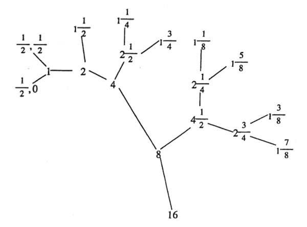
Now the intersection of these two groups is the modular subgroup $\Gamma_0(N) $ (consisting of those modular group element whose lower left-hand entry is divisible by N). That is, the proper way to look at this arithmetic group is as the joint stabilizer of the two lattices $L_1,L_N $. The picture makes it trivial to compute the index of this subgroup.

Consider the ball $B(L_1,N) $ with center $L_1 $ and hyper-radius N (on the left, the ball with hyper-radius 4). Then, it is easy to show that the modular group acts transitively on the boundary lattices (including the lattice $L_N $), whence the index $[ \Gamma : \Gamma_0(N)] $ is just the number of these boundary lattices. For N=4 the picture shows that there are exactly 6 of them. In general, it follows from our knowledge of all the p-trees the number of all lattices at hyperdistance N from $L_1 $ is equal to $N \prod_{p | N}(1+ \frac{1}{p}) $, in accordance with the well-known index formula for these modular subgroups!

But, there are many other applications of the big picture giving a simple interpretation for the Hecke operators, an elegant proof of the Atkin-Lehner theorem on the normalizer of $\Gamma_0(N) $ (the whimsical source of appearances of the number 24) and of Helling’s theorem characterizing maximal arithmetical groups inside $PSL_2(\mathbb{C}) $ as conjugates of the normalizers of $\Gamma_0(N) $ for square-free N.
J.H. Conway’s paper “Understanding groups like $\Gamma_0(N) $” containing all this material is a must-read! Unfortunately, I do not know of an online version.

the monster graph and McKay’s observation

Published April 22, 2009 by lievenlb

While the verdict on a neolithic Scottish icosahedron is still open, let us recall Kostant’s group-theoretic construction of the icosahedron from its rotation-symmetry group $A_5 $.

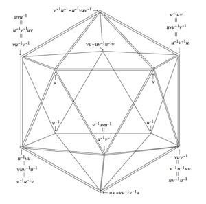The alternating group $A_5 $ has two conjugacy classes of order 5 elements, both consisting of exactly 12 elements. Fix one of these conjugacy classes, say $C $ and construct a graph with vertices the 12 elements of $C $ and an edge between two $u,v \in C $ if and only if the group-product $u.v \in C $ still belongs to the same conjugacy class.

Observe that this relation is symmetric as from $u.v = w \in C $ it follows that $v.u=u^{-1}.u.v.u = u^{-1}.w.u \in C $. The graph obtained is the icosahedron, depicted on the right with vertices written as words in two adjacent elements u and v from $C $, as indicated.

Kostant writes : “Normally it is not a common practice in group theory to consider whether or not the product of two elements in a conjugacy class is again an element in that conjugacy class. However such a consideration here turns out to be quite productive.”

Still, similar constructions have been used in other groups as well, in particular in the study of the largest sporadic group, the monster group $\mathbb{M} $.

There is one important catch. Whereas it is quite trivial to multiply two permutations and verify whether the result is among 12 given ones, for most of us mortals it is impossible to do actual calculations in the monster. So, we’d better have an alternative way to get at the icosahedral graph using only $A_5 $-data that is also available for the monster group, such as its character table.

Let $G $ be any finite group and consider three of its conjugacy classes $C(i),C(j) $ and $C(k) $. For any element $w \in C(k) $ we can compute from the character table of $G $ the number of different products $u.v = w $ such that $u \in C(i) $ and $v \in C(j) $. This number is given by the formula

$\frac{|G|}{|C_G(g_i)||C_G(g_j)|} \sum_{\chi} \frac{\chi(g_i) \chi(g_j) \overline{\chi(g_k)}}{\chi(1)} $

where the sum is taken over all irreducible characters $\chi $ and where $g_i \in C(i),g_j \in C(j) $ and $g_k \in C(k) $. Note also that $|C_G(g)| $ is the number of $G $-elements commuting with $g $ and that this number is the order of $G $ divided by the number of elements in the conjugacy class of $g $.

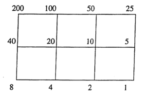
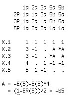The character table of $A_5 $ is given on the left : the five columns correspond to the different conjugacy classes of elements of order resp. 1,2,3,5 and 5 and the rows are the character functions of the 5 irreducible representations of dimensions 1,3,3,4 and 5.

Let us fix the 4th conjugacy class, that is 5a, as our class $C $. By the general formula, for a fixed $w \in C $ the number of different products $u.v=w $ with $u,v \in C $ is equal to

$\frac{60}{25}(\frac{1}{1} + \frac{(\frac{1+\sqrt{5}}{2})^3}{3} + \frac{(\frac{1-\sqrt{5}}{2})^3}{3} – \frac{1}{4} + \frac{0}{5}) = \frac{60}{25}(1 + \frac{4}{3} – \frac{1}{4}) = 5 $

Because for each $x \in C $ also its inverse $x^{-1} \in C $, this can be rephrased by saying that there are exactly 5 different products $w^{-1}.u \in C $, or equivalently, that the valency of every vertex $w^{-1} \in C $ in the graph is exactly 5.

That is, our graph has 12 vertices, each with exactly 5 neighbors, and with a bit of extra work one can show it to be the icosahedral graph.

For the monster group, the Atlas tells us that it has exactly 194 irreducible representations (and hence also 194 conjugacy classes). Of these conjugacy classes, the involutions (that is the elements of order 2) are of particular importance.

There are exactly 2 conjugacy classes of involutions, usually denoted 2A and 2B. Involutions in class 2A are called “Fischer-involutions”, after Bernd Fischer, because their centralizer subgroup is an extension of Fischer’s baby Monster sporadic group.

Likewise, involutions in class 2B are usually called “Conway-involutions” because their centralizer subgroup is an extension of the largest Conway sporadic group.

Let us define the monster graph to be the graph having as its vertices the Fischer-involutions and with an edge between two of them $u,v \in 2A $ if and only if their product $u.v $ is again a Fischer-involution.

Because the centralizer subgroup is $2.\mathbb{B} $, the number of vertices is equal to $97239461142009186000 = 2^4 * 3^7 * 5^3 * 7^4 * 11 * 13^2 * 29 * 41 * 59 * 71 $.

From the general result recalled before we have that the valency in all vertices is equal and to determine it we have to use the character table of the monster and the formula. Fortunately GAP provides the function ClassMultiplicationCoefficient to do this without making errors.

gap> table:=CharacterTable("M"); CharacterTable( "M" ) gap> ClassMultiplicationCoefficient(table,2,2,2); 27143910000

Perhaps noticeable is the fact that the prime decomposition of the valency $27143910000 = 2^4 * 3^4 * 5^4 * 23 * 31 * 47 $ is symmetric in the three smallest and three largest prime factors of the baby monster order.

Robert Griess proved that one can recover the monster group $\mathbb{M} $ from the monster graph as its automorphism group!

As in the case of the icosahedral graph, the number of vertices and their common valency does not determine the monster graph uniquely. To gain more insight, we would like to know more about the sizes of minimal circuits in the graph, the number of such minimal circuits going through a fixed vertex, and so on.

Such an investigation quickly leads to a careful analysis which other elements can be obtained from products $u.v $ of two Fischer involutions $u,v \in 2A $. We are in for a major surprise, first observed by John McKay:

Printing out the number of products of two Fischer-involutions giving an element in the i-th conjugacy class of the monster,
where i runs over all 194 possible classes, we get the following string of numbers :

97239461142009186000, 27143910000, 196560, 920808, 0, 3, 1104, 4, 0, 0, 5, 0, 6, 0, 0, 0, 0, 0, 0, 0, 0, 0, 0, 0, 0, 0, 0, 0, 0, 0, 0, 0, 0, 0, 0, 0, 0, 0, 0, 0, 0, 0, 0, 0, 0, 0, 0, 0, 0, 0, 0, 0, 0, 0, 0, 0, 0, 0, 0, 0, 0, 0, 0, 0, 0, 0, 0, 0, 0, 0, 0, 0, 0, 0, 0, 0, 0, 0, 0, 0, 0, 0, 0, 0, 0, 0, 0, 0, 0, 0, 0, 0, 0, 0, 0, 0, 0, 0, 0, 0, 0, 0, 0, 0, 0, 0, 0, 0, 0, 0, 0, 0, 0, 0, 0, 0, 0, 0, 0, 0, 0, 0, 0, 0, 0, 0, 0, 0, 0, 0, 0, 0, 0, 0, 0, 0, 0, 0, 0, 0, 0, 0, 0, 0, 0, 0, 0, 0, 0, 0, 0, 0, 0, 0, 0, 0, 0, 0, 0, 0, 0, 0, 0, 0, 0, 0, 0, 0, 0, 0, 0, 0, 0, 0, 0, 0, 0, 0, 0, 0, 0, 0, 0, 0, 0, 0, 0, 0, 0, 0, 0, 0, 0, 0

That is, the elements of only 9 conjugacy classes can be written as products of two Fischer-involutions! These classes are :

1A = { 1 } written in 97239461142009186000 different ways (after all involutions have order two)
2A, each element of which can be written in exactly 27143910000 different ways (the valency)
2B, each element of which can be written in exactly 196560 different ways. Observe that this is the kissing number of the Leech lattice leading to a permutation representation of $2.Co_1 $.
3A, each element of which can be written in exactly 920808 ways. Note that this number gives a permutation representation of the maximal monster subgroup $3.Fi_{24}’ $.
3C, each element of which can be written in exactly 3 ways.
4A, each element of which can be written in exactly 1104 ways.
4B, each element of which can be written in exactly 4 ways.
5A, each element of which can be written in exactly 5 ways.
6A, each element of which can be written in exactly 6 ways.

Let us forget about the actual numbers for the moment and concentrate on the orders of these 9 conjugacy classes : 1,2,2,3,3,4,4,5,6. These are precisely the components of the fundamental root of the extended Dynkin diagram $\tilde{E_8} $!

This is the content of John McKay’s E(8)-observation : there should be a precise relation between the nodes of the extended Dynkin diagram and these 9 conjugacy classes in such a way that the order of the class corresponds to the component of the fundamental root. More precisely, one conjectures the following correspondence

This is similar to the classical McKay correspondence between finite subgroups of $SU(2) $ and extended Dynkin diagrams (the binary icosahedral group corresponding to extended E(8)). In that correspondence, the nodes of the Dynkin diagram correspond to irreducible representations of the group and the edges are determined by the decompositions of tensor-products with the fundamental 2-dimensional representation.

Here, however, the nodes have to correspond to conjugacy classes (rather than representations) and we have to look for another procedure to arrive at the required edges! An exciting proposal has been put forward recently by John Duncan in his paper Arithmetic groups and the affine E8 Dynkin diagram.

It will take us a couple of posts to get there, but for now, let’s give the gist of it : monstrous moonshine gives a correspondence between conjugacy classes of the monster and certain arithmetic subgroups of $PSL_2(\mathbb{R}) $ commensurable with the modular group $\Gamma = PSL_2(\mathbb{Z}) $. The edges of the extended Dynkin E(8) diagram are then given by the configuration of the arithmetic groups corresponding to the indicated 9 conjugacy classes! (to be continued…)