Skip to content →

Tag: Lenstra

A suit with shorts

I’m retiring in two weeks so I’m cleaning out my office.

So far, I got rid of almost all paper-work and have split my book-collection in two: the books I want to take with me, and those anyone can grab away.

Here’s the second batch (math/computer books in the middle, popular science to the right, thrillers to the left).


If you’re interested in some of these books (click for a larger image, if you want to zoom in) and are willing to pay the postage, leave a comment and I’ll try to send them if they survive the current ‘take-away’ phase.

Here are two books I definitely want to keep. On the left, an original mimeographed version of Mumford’s ‘Red Book’.

On the right, ‘Een pak met een korte broek’ (‘A suit with shorts’), a collection of papers by family and friends, presented to Hendrik Lenstra on the occasion of the defence of his Ph.D. thesis on Euclidean number-fields, May 18th 1977.

If the title intrigues you, a photo of young Hendrik in suit and shorts is included.

This collection includes hilarious ‘papers’ by famous people including

  • ‘A headache-causing problem’ by Conway (J.H.), Paterson (M.S.), and Moscow (U.S.S.R.)
  • ‘A projective plain of order ten’ by A.M. Odlyzko and N.J.A. Sloane
  • ‘La chasse aux anneaux principaux non-Euclidiens dans l’enseignement’ by Pierre Samuel
  • ‘On time-like theorems’ by Michiel Hazewinkel
  • ‘She loves me, she loves me not’ by Richard K. Guy
  • ‘Theta invariants for affine root systems’ by E.J.N. Looijenga
  • ‘The prime of primes’ by F. Lenstra and A.J. Oort
  • (and many more, most of them in Dutch)

Perhaps I can do a couple of posts on some of these papers. It might break this clean-up routine.

One Comment

How to play Nimbers?

Nimbers is a 2-person game, winnable only if you understand the arithmetic of the finite fields $\mathbb{F}_{2^{2^n}} $ associated to Fermat 2-powers.

It is played on a rectangular array (say a portion of a Go-board, for practical purposes) having a finite number of stones at distinct intersections. Here’s a typical position

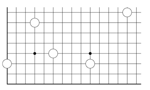
The players alternate making a move, which is either

  • removing one stone, or
  • moving a stone to a spot on the same row (resp. the same column) strictly to the left (resp. strictly lower), and if there’s already a stone on this spot, both stones are removed, or
  • adding stones to the empty corners of a rectangle having as its top-right hand corner a chosen stone and removing stones at the occupied corners

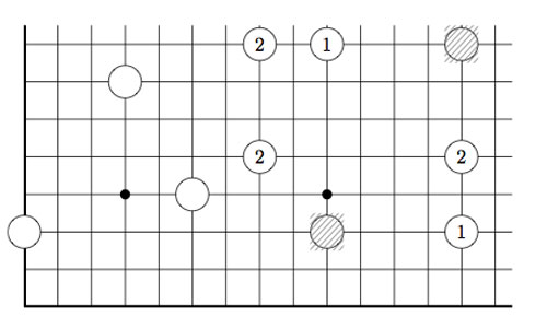
Here we illustrate two possible moves from the above position, in the first we add two new stones and remove 2 existing stones, in the second we add three new stones and remove only the top right-hand stone.

As always, the last player able to move wins the game!

Note that Nimbers is equivalent to Lenstra’s ‘turning corners’-game (as introduced in his paper Nim-multiplication or mentioned in Winning Ways Chapter 14, page 473).

If all stones are placed on the left-most column (or on the bottom row) one quickly realizes that this game reduces to classical Nim with Nim-heap sizes corresponding to the stones (for example, the left-most stone corresponds to a heap of size 3).

Nim-addition $n \oplus m $ is defined inductively by

$n \oplus m = mex(n’ \oplus m,n \oplus m’) $

where $n’ $ is any element of ${ 0,1,\ldots,n-1 } $ and $m’ $ any element of ${ 0,1,\ldots,m-1 } $ and where ‘mex’ stands for Minimal EXcluded number, that is the smallest natural number which isn’t included in the set. Alternatively, one can compute $n \oplus m $ buy writing $n $ and $m $ in binary and add these binary numbers without carrying-over. It is well known that a winning strategy for Nim tries to shorten one Nim-heap such that the Nim-addition of the heap-sizes equals zero.

This allows us to play Nimber-endgames, that is, when all the stones have been moved to the left-column or the bottom row.

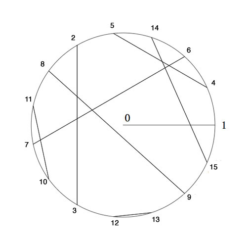
To evaluate general Nimber-positions it is best to add another row and column, the coordinate axes of the array

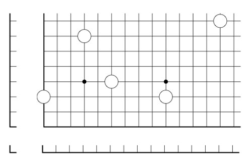
and so our stones lie at positions (1,3), (4,7), (6,4), (10,3) and (14,8). In this way all legal moves follow the rectangle-rule when we allow rectangles to contain corners on the added coordinate axes. For example, removing a stone is achieved by taking a rectangle with two sides on the added axes, and, moving a stone to the left (or the bottom) is done by taking a rectangle with one side at the x-axes (resp. the y-axes)

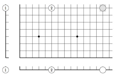
However, the added stones on the coordinate axes are considered dead and may be removed from the game. This observation allows us to compute the Grundy number of a stone at position (m,n) to be

$G(m,n)=mex(G(m’,n’) \oplus G(m’,n) \oplus G(m,n’)~:~0 \leq m’ < m, 0 \leq n’ < n) $

and so by induction these Grundy numbers are equal to the Nim-multiplication $G(m,n) = m \otimes n $ where

$m \otimes n = mex(m’ \otimes n’ \oplus m’ \otimes n \oplus m \otimes n’~:~0 \leq m’ < m, 0 \leq n’ < n) $

Thus, we can evaluate any Nimbers-position with stone-coordinates smaller than $2^{2^n} $ by calculating in a finite field using the identification (as for example in the odd Knights of the round table-post) $\mathbb{F}_{2^{2^n}} = \{ 0,1,2,\ldots,2^{2^n}-1 \} $

For example, when all stones lie in a 15×15 grid (as in the example above), all calculations can be performed using

Here, we’ve identified the non-zero elements of $\mathbb{F}_{16} $ with 15-th roots of unity, allowing us to multiply, and we’ve paired up couples $(n,n \oplus 1) $ allowing u to reduce nim-addition to nim-multiplication via

$n \oplus m = (n \otimes \frac{1}{m}) \otimes (m \oplus 1) $

In particular, the stone at position (14,8) is equivalent to a Nim-heap of size $14 \otimes 8=10 $. The nim-value of the original position is equal to 8

Suppose your opponent lets you add one extra stone along the diagonal if you allow her to start the game, where would you have to place it and be certain you will win the game?

One Comment

Lambda-rings for formula-phobics

In 1956, Alexander Grothendieck (middle) introduced $\lambda $-rings in an algebraic-geometric context to be commutative rings A equipped with a bunch of operations $\lambda^i $ (for all numbers $i \in \mathbb{N}_+ $) satisfying a list of rather obscure identities. From the easier ones, such as

$\lambda^0(x)=1, \lambda^1(x)=x, \lambda^n(x+y) = \sum_i \lambda^i(x) \lambda^{n-i}(y) $

to those expressing $\lambda^n(x.y) $ and $\lambda^m(\lambda^n(x)) $ via specific universal polynomials. An attempt to capture the essence of $\lambda $-rings without formulas?

Lenstra’s elegant construction of the 1-power series rings $~(\Lambda(A),\oplus,\otimes) $ requires only one identity to remember

$~(1-at)^{-1} \otimes (1-bt)^{-1} = (1-abt)^{-1} $.

Still, one can use it to show the existence of ringmorphisms $\gamma_n~:~\Lambda(A) \rightarrow A $, for all numbers $n \in \mathbb{N}_+ $. Consider the formal ‘logarithmic derivative’

$\gamma = \frac{t u(t)’}{u(t)} = \sum_{i=1}^\infty \gamma_i(u(t))t^i~:~\Lambda(A) \rightarrow A[[t]] $

where $u(t)’ $ is the usual formal derivative of a power series. As this derivative satisfies the chain rule, we have

$\gamma(u(t) \oplus v(t)) = \frac{t (u(t)v(t))’}{u(t)v(t)} = \frac{t(u(t)’v(t)+u(t)v(t)’}{u(t)v(t))} = \frac{tu(t)’}{u(t)} + \frac{tv(t)’}{v(t)} = \gamma(u(t)) + \gamma(v(t)) $

and so all the maps $\gamma_n~:~\Lambda(A) \rightarrow A $ are additive. To show that they are also multiplicative, it suffices by functoriality to verify this on the special 1-series $~(1-at)^{-1} $ for all $a \in A $. But,

$\gamma((1-at)^{-1}) = \frac{t \frac{a}{(1-at)^2}}{(1-at)} = \frac{at}{(1-at)} = at + a^2t^2 + a^3t^3+\ldots $

That is, $\gamma_n((1-at)^{-1}) = a^n $ and Lenstra’s identity implies that $\gamma_n $ is indeed multiplicative! A first attempt :

hassle-free definition 1 : a commutative ring $A $ is a $\lambda $-ring if and only if there is a ringmorphism $s_A~:~A \rightarrow \Lambda(A) $ splitting $\gamma_1 $, that is, such that $\gamma_1 \circ s_A = id_A $.

In particular, a $\lambda $-ring comes equipped with a multiplicative set of ring-endomorphisms $s_n = \gamma_n \circ s_A~:~A \rightarrow A $ satisfying $s_m \circ s_m = s_{mn} $. One can then define a $\lambda $-ringmorphism to be a ringmorphism commuting with these endo-morphisms.

The motivation being that $\lambda $-rings are known to form a subcategory of commutative rings for which the 1-power series functor is the right adjoint to the functor forgetting the $\lambda $-structure. In particular, if $A $ is a $\lambda $-ring, we have a ringmorphism $A \rightarrow \Lambda(A) $ corresponding to the identity morphism.

But then, what is the connection to the usual one involving all the operations $\lambda^i $? Well, one ought to recover those from $s_A(a) = (1-\lambda^1(a)t+\lambda^2(a)t^2-\lambda^3(a)t^3+…)^{-1} $.

For $s_A $ to be a ringmorphism will require identities among the $\lambda^i $. I hope an expert will correct me on this one, but I’d guess we won’t yet obtain all identities required. By the very definition of an adjoint we must have that $s_A $ is a morphism of $\lambda $-rings, and, this would require defining a $\lambda $-ring structure on $\Lambda(A) $, that is a ringmorphism $s_{AH}~:~\Lambda(A) \rightarrow \Lambda(\Lambda(A)) $, the so called Artin-Hasse exponential, to which I’d like to return later.

For now, we can define a multiplicative set of ring-endomorphisms $f_n~:~\Lambda(A) \rightarrow \Lambda(A) $ from requiring that $f_n((1-at)^{-1}) = (1-a^nt)^{-1} $ for all $a \in A $. Another try?

hassle-free definition 2 : $A $ is a $\lambda $-ring if and only if there is splitting $s_A $ to $\gamma_1 $ satisfying the compatibility relations $f_n \circ s_A = s_A \circ s_n $.

But even then, checking that a map $s_A~:~A \rightarrow \Lambda(A) $ is a ringmorphism is as hard as verifying the lists of identities among the $\lambda^i $. Fortunately, we get such a ringmorphism for free in the important case when A is of ‘characteristic zero’, that is, has no additive torsion. Then, a ringmorphism $A \rightarrow \Lambda(A) $ exists whenever we have a multiplicative set of ring endomorphisms $F_n~:~A \rightarrow A $ for all $n \in \mathbb{N}_+ $ such that for every prime number $p $ the morphism $F_p $ is a lift of the Frobenius, that is, $F_p(a) \in a^p + pA $.

Perhaps this captures the essence of $\lambda $-rings best (without the risk of getting an headache) : in characteristic zero, they are the (commutative) rings having a multiplicative set of endomorphisms, generated by lifts of the Frobenius maps.

2 Comments

big Witt vectors for everyone (1/2)

Next time you visit your math-library, please have a look whether these books are still on the shelves : Michiel Hazewinkel‘s Formal groups and applications, William Fulton’s and Serge Lange’s Riemann-Roch algebra and Donald Knutson’s lambda-rings and the representation theory of the symmetric group.

I wouldn’t be surprised if one or more of these books are borrowed out, probably all of them to the same person. I’m afraid I’m that person in Antwerp…

Lately, there’s been a renewed interest in $\lambda $-rings and the endo-functor W assigning to a commutative algebra its ring of big Witt vectors, following Borger’s new proposal for a geometry over the absolute point.

However, as Hendrik Lenstra writes in his 2002 course-notes on the subject Construction of the ring of Witt vectors : “The literature on the functor W is in a somewhat unsatisfactory state: nobody seems to have any interest in Witt vectors beyond applying them for a purpose, and they are often treated in appendices to papers devoting to something else; also, the construction usually depends on a set of implicit or unintelligible formulae. Apparently, anybody who wishes to understand Witt vectors needs to construct them personally. That is what is now happening to myself.”

Before doing a series on Borger’s paper, we’d better run through Lenstra’s elegant construction in a couple of posts. Let A be a commutative ring and consider the multiplicative group of all ‘one-power series’ over it $\Lambda(A)=1+t A[[t]] $. Our aim is to define a commutative ring structure on $\Lambda(A) $ taking as its ADDITION the MULTIPLICATION of power series.

That is, if $u(t),v(t) \in \Lambda(A) $, then we define our addition $u(t) \oplus v(t) = u(t) \times v(t) $. This may be slightly confusing as the ZERO-element in $\Lambda(A),\oplus $ will then turn be the constant power series 1…

We are now going to define a multiplication $\otimes $ on $\Lambda(A) $ which is distributively with respect to $\oplus $ and turns $\Lambda(A) $ into a commutative ring with ONE-element the series $~(1-t)^{-1}=1+t+t^2+t^3+\ldots $.

We will do this inductively, so consider $\Lambda_n(A) $ the (classes of) one-power series truncated at term n, that is, the kernel of the natural augmentation map between the multiplicative group-units $~A[t]/(t^{n+1})^* \rightarrow A^* $.
Again, taking multiplication in $A[t]/(t^{n+1}) $ as a new addition rule $\oplus $, we see that $~(\Lambda_n(A),\oplus) $ is an Abelian group, whence a $\mathbb{Z} $-module.

For all elements $a \in A $ we have a scaling operator $\phi_a $ (sending $t \rightarrow at $) which is an A-ring endomorphism of $A[t]/(t^{n+1}) $, in particular multiplicative wrt. $\times $. But then, $\phi_a $ is an additive endomorphism of $~(\Lambda_n(A),\oplus) $, so is an element of the endomorphism-RING $End_{\mathbb{Z}}(\Lambda_n(A)) $. Because composition (being the multiplication in this endomorphism ring) of scaling operators is clearly commutative ($\phi_a \circ \phi_b = \phi_{ab} $) we can define a commutative RING $E $ being the subring of $End_{\mathbb{Z}}(\Lambda_n(A)) $ generated by the operators $\phi_a $.

The action turns $~(\Lambda_n(A),\oplus) $ into an E-module and we define an E-module morphism $E \rightarrow \Lambda_n(A) $ by $\phi_a \mapsto \phi_a((1-t)^{-1}) = (1-at)^{-a} $.

All of this looks pretty harmless, but the upshot is that we have now equipped the image of this E-module morphism, say $L_n(A) $ (which is the additive subgroup of $~(\Lambda_n(A),\oplus) $ generated by the elements $~(1-at)^{-1} $) with a commutative multiplication $\otimes $ induced by the rule $~(1-at)^{-1} \otimes (1-bt)^{-1} = (1-abt)^{-1} $.

Explicitly, $L_n(A) $ is the set of one-truncated polynomials $u(t) $ with coefficients in $A $ such that one can find elements $a_1,\ldots,a_k \in A $ such that $u(t) \equiv (1-a_1t)^{-1} \times \ldots \times (1-a_k)^{-1}~mod~t^{n+1} $. We multiply $u(t) $ with another such truncated one-polynomial $v(t) $ (taking elements $b_1,b_2,\ldots,b_l \in A $) via

$u(t) \otimes v(t) = ((1-a_1t)^{-1} \oplus \ldots \oplus (1-a_k)^{-1}) \otimes ((1-b_1t)^{-1} \oplus \ldots \oplus (1-b_l)^{-1}) $

and using distributivity and the multiplication rule this gives the element $\prod_{i,j} (1-a_ib_jt)^{-1}~mod~t^{n+1} \in L_n(A) $.
Being a ring-qutient of $E $ we have that $~(L_n(A),\oplus,\otimes) $ is a commutative ring, and, from the construction it is clear that $L_n $ behaves functorially.

For rings $A $ such that $L_n(A)=\Lambda_n(A) $ we are done, but in general $L_n(A) $ may be strictly smaller. The idea is to use functoriality and do the relevant calculations in a larger ring $A \subset B $ where we can multiply the two truncated one-polynomials and observe that the resulting truncated polynomial still has all its coefficients in $A $.

Here’s how we would do this over $\mathbb{Z} $ : take two irreducible one-polynomials u(t) and v(t) of degrees r resp. s smaller or equal to n. Then over the complex numbers we have
$u(t)=(1-\alpha_1t) \ldots (1-\alpha_rt) $ and $v(t)=(1-\beta_1) \ldots (1-\beta_st) $. Then, over the field $K=\mathbb{Q}(\alpha_1,\ldots,\alpha_r,\beta_1,\ldots,\beta_s) $ we have that $u(t),v(t) \in L_n(K) $ and hence we can compute their product $u(t) \otimes v(t) $ as before to be $\prod_{i,j}(1-\alpha_i\beta_jt)^{-1}~mod~t^{n+1} $. But then, all coefficients of this truncated K-polynomial are invariant under all permutations of the roots $\alpha_i $ and the roots $\beta_j $ and so is invariant under all elements of the Galois group. But then, these coefficients are algebraic numbers in $\mathbb{Q} $ whence integers. That is, $u(t) \otimes v(t) \in \Lambda_n(\mathbb{Z}) $. It should already be clear from this that the rings $\Lambda_n(\mathbb{Z}) $ contain a lot of arithmetic information!

For a general commutative ring $A $ we will copy this argument by considering a free overring $A^{(\infty)} $ (with 1 as one of the base elements) by formally adjoining roots. At level 1, consider $M_0 $ to be the set of all non-constant one-polynomials over $A $ and consider the ring

$A^{(1)} = \bigotimes_{f \in M_0} A[X]/(f) = A[X_f, f \in M_0]/(f(X_f) , f \in M_0) $

The idea being that every one-polynomial $f \in M_0 $ now has one root, namely $\alpha_f = \overline{X_f} $ in $A^{(1)} $. Further, $A^{(1)} $ is a free A-module with basis elements all $\alpha_f^i $ with $0 \leq i < deg(f) $.

Good! We now have at least one root, but we can continue this process. At level 2, $M_1 $ will be the set of all non-constant one-polynomials over $A^{(1)} $ and we use them to construct the free overring $A^{(2)} $ (which now has the property that every $f \in M_0 $ has at least two roots in $A^{(2)} $). And, again, we repeat this process and obtain in succession the rings $A^{(3)},A^{(4)},\ldots $. Finally, we define $A^{(\infty)} = \underset{\rightarrow}{lim}~A^{(i)} $ having the property that every one-polynomial over A splits entirely in linear factors over $A^{(\infty)} $.

But then, for all $u(t),v(t) \in \Lambda_n(A) $ we can compute $u(t) \otimes v(t) \in \Lambda_n(A^{(\infty)}) $. Remains to show that the resulting truncated one-polynomial has all its entries in A. The ring $A^{(\infty)} \otimes_A A^{(\infty)} $ contains two copies of $A^{(\infty)} $ namely $A^{(\infty)} \otimes 1 $ and $1 \otimes A^{(\infty)} $ and the intersection of these two rings in exactly $A $ (here we use the freeness property and the additional fact that 1 is one of the base elements). But then, by functoriality of $L_n $, the element
$u(t) \otimes v(t) \in L_n(A^{(\infty)} \otimes_A A^{(\infty)}) $ lies in the intersection $\Lambda_n(A^{(\infty)} \otimes 1) \cap \Lambda_n(1 \otimes A^{(\infty)})=\Lambda_n(A) $. Done!

Hence, we have endo-functors $\Lambda_n $ in the category of all commutative rings, for every number n. Reviewing the construction of $L_n $ one observes that there are natural transformations $L_{n+1} \rightarrow L_n $ and therefore also natural transformations $\Lambda_{n+1} \rightarrow \Lambda_n $. Taking the inverse limits $\Lambda(A) = \underset{\leftarrow}{lim} \Lambda_n(A) $ we therefore have the ‘one-power series’ endo-functor
$\Lambda~:~\mathbf{comm} \rightarrow \mathbf{comm} $
which is ‘almost’ the functor W of big Witt vectors. Next time we’ll take you through the identification using ‘ghost variables’ and how the functor $\Lambda $ can be used to define the category of $\lambda $-rings.

One Comment

On2 : extending Lenstra’s list

We have seen that John Conway defined a nim-addition and nim-multiplication on the ordinal numbers in such a way that the subfield $[\omega^{\omega^{\omega}}] \simeq \overline{\mathbb{F}}_2 $ is the algebraic closure of the field on two elements. We’ve also seen how to do actual calculations in that field provided we can determine the mystery elements $\alpha_p $, which are the smallest ordinals not being a p-th power of ordinals lesser than $[\omega^{\omega^{k-1}}] $ if $p $ is the $k+1 $-th prime number.

Hendrik Lenstra came up with an effective method to compute these elements $\alpha_p $ requiring a few computations in certain finite fields. I’ll give a rundown of his method and refer to his 1977-paper “On the algebraic closure of two” for full details.

For any ordinal $\alpha < \omega^{\omega^{\omega}} $ define its degree $d(\alpha) $ to be the degree of minimal polynomial for $\alpha $ over $\mathbb{F}_2 = [2] $ and for each prime number $p $ let $f(p) $ be the smallest number $h $ such that $p $ is a divisor of $2^h-1 $ (clearly $f(p) $ is a divisor of $p-1 $).

In the previous post we have already defined ordinals $\kappa_{p^k}=[\omega^{\omega^{k-1}.p^{n-1}}] $ for prime-power indices, but we now need to extend this definition to allow for all indices. So. let $h $ be a natural number, $p $ the smallest prime number dividing $h $ and $q $ the highest power of $p $ dividing $h $. Let $g=[h/q] $, then Lenstra defines

$\kappa_h = \begin{cases} \kappa_q~\text{if q divides}~d(\kappa_q)~\text{ and} \\ \kappa_g + \kappa_q = [\kappa_g + \kappa_q]~\text{otherwise} \end{cases} $

With these notations, the main result asserts the existence of natural numbers $m,m’ $ such that

$\alpha_p = [\kappa_{f(p)} + m] = [\kappa_{f(p)}] + m’ $

Now, assume by induction that we have already determined the mystery numbers $\alpha_r $ for all odd primes $r < p $, then by teh argument of last time we can effectively compute in the field $[\kappa_p] $. In particular, we can compute for every element its multiplicative order $ord(\beta) $ and therefore also its degree $d(\beta) $ which has to be the smallest number $h $ such that $ord(\beta) $ divides $[2^h-1] $.

Then, by the main result we only have to determine the smallest number m such that $\beta = [\kappa_{f(p)} +m] $ is not a p-th power in $\kappa_p $ which is equivalent to the condition that

$\beta^{(2^{d(\beta)}-1)/p} \not= 1 $ if $p $ divides $[2^{d(\beta)}-1] $

All these conditions can be verified within suitable finite fields and hence are effective. In this manner, Lenstra could extend Conway’s calculations (probably using a home-made finite field program running on a slow 1977 machine) :

[tex]\begin{array}{c|c|c} p & f(p) & \alpha_p \\ \hline 3 & 2 & [2] \\ 5 & 4 & [4] \\ 7 & 3 & [\omega]+1 \\ 11 & 10 & [\omega^{\omega}]+1 \\ 13 & 12 & [\omega]+4 \\ 17 & 8 & [16] \\ 19 & 18 & [\omega^3]+4 \\ 23 & 11 & [\omega^{\omega^3}]+1 \\ 29 & 28 & [\omega^{\omega^2}]+4 \\ 31 & 5 & [\omega^{\omega}]+1 \\ 37 & 36 & [\omega^3]+4 \\ 41 & 20 & [\omega^{\omega}]+1 \\ 43 & 14 & [\omega^{\omega^2}]+ 1 \end{array}[/tex]

Right, so let’s try the case $p=47 $. To begin, $f(47)=23 $ whence we have to determine the smallest field containg $\kappa_{23} $. By induction (Lenstra’s tabel) we know already that

$\kappa_{23}^{23} = \kappa_{11} + 1 = [\omega^{\omega^3}]+1 $ and $\kappa_{11}^{11} = \kappa_5 + 1 = [\omega^{\omega}]+1 $ and $\kappa_5^5=[4] $

Because the smallest field containg $4 $ is $[16]=\mathbb{F}_{2^4} $ we have that $\mathbb{F}_2(4,\kappa_5,\kappa_{11}) \simeq \mathbb{F}_{2^{220}} $. We can construct this finite field, together with a generator $a $ of its multiplicative group in Sage via


sage: f1.< a >=GF(2^220)

In this field we have to pinpoint the elements $4,\kappa_5 $ and $\kappa_{11} $. As $4 $ has order $15 $ in $\mathbb{F}_{2^4} $ we know that $\kappa_5 $ has order $75 $. Hence we can take $\kappa_5 = a^{(2^{220}-1)/75} $ and then $4=\kappa_5^5 $.

If we denote $\kappa_5 $ by x5 we can obtain $\kappa_{11} $ as x11 by the following sage-commands


sage: c=x5+1

sage: x11=c.nth_root(11)

It takes about 7 minutes to find x11 on a 2.4 GHz MacBook. Next, we have to set up the field extension determined by $\kappa_{23} $ (which we will call x in sage). This is done as follows


sage: p1.=PolynomialRing(f1)

sage: f=x^23-x11-1

sage: F2=f1.extension(f,'u')

The MacBook needed 8 minutes to set up this field which is isomorphic to $\mathbb{F}_{2^{5060}} $. The relevant number is therefore $n=\frac{2^{5060}-1}{47} $ which is the gruesome

34648162040462867047623719793206539850507437636617898959901744136581<br/>
259144476645069239839415478030722644334257066691823210120548345667203443<br/>
317743531975748823386990680394012962375061822291120459167399032726669613
<br/>
442804392429947890878007964213600720766879334103454250982141991553270171

938532417844211304203805934829097913753132491802446697429102630902307815

301045433019807776921086247690468136447620036910689177286910624860871748

150613285530830034500671245400628768674394130880959338197158054296625733

206509650361461537510912269982522844517989399782602216622257291361930850

885916974186835958466930689748400561295128553674118498999873244045842040

080195019701984054428846798610542372150816780493166669821114184374697446

637066566831036116390063418916814141753876530004881539570659100352197393

997895251223633176404672792711603439161147155163219282934597310848529360

118189507461132290706604796116111868096099527077437183219418195396666836

014856037176421475300935193266597196833361131333604528218621261753883518

667866835204501888103795022437662796445008236823338104580840186181111557

498232520943552183185687638366809541685702608288630073248626226874916669

186372183233071573318563658579214650042598011275864591248749957431967297

975078011358342282941831582626985121760847852546207377440873367589369439

085660784239080183415569559585998884824991911321095149718147110882474280

968166266224151511519773175933506503369761671964823112231808283557885030

984081329986188655169245595411930535264918359325712373064120338963742590

76555755141425

Remains ‘only’ to take x,x+1,etc. to the n-th power and verify which is the first to be unequal to 1. For this it is best to implement the usual powering trick (via digital expression of the exponent) in the field F2, something like


sage: def power(e,n):
...: le=n.bits()
...: v=n.digits()
...: mn=F2(e)
...: out=F2(1)
...: i=0
...: while i< le :
...: if v[i]==1 : out=F2(out_mn)
...: m=F2(mn_mn)
...: mn=F2(m)
...: i=i+1
...: return(out)
...:

then it takes about 20 seconds to verify that power(x,n)=1 but that power(x+1,n) is NOT! That is, we just checked that $\alpha_{47}=\kappa_{11}+1 $.

It turns out that 47 is the hardest nut to crack, the following primes are easier. Here’s the data (if I didn’t make mistakes…)

[tex]\begin{array}{c|c|c} p & f(p) & \alpha_p \\ \hline 47 & 23 & [\omega^{\omega^{7}}]+1 \\ 53 & 52 & [\omega^{\omega^4}]+1 \\ 59 & 58 & [\omega^{\omega^8}]+1 \\ 61 & 60 & [\omega^{\omega}]+[\omega] \\ 67 & 66 & [\omega^{\omega^3}]+[\omega] \end{array}[/tex]

It seems that Magma is substantially better at finite field arithmetic, so if you are lucky enough to have it you’ll have no problem finding $\alpha_p $ for all primes less than 100 by the end of the day. If you do, please drop a comment with the results…

Leave a Comment

5 years blogging

Here’s a 5 move game from $\mathbb{C} $, the complex numbers game, annotated by Hendrik Lenstra in Nim multiplication.

$\begin{matrix} & \text{White} & \text{Black} \\ 1. & 3-2i & { 3_{\mathbb{R}} } \\ 2. & 3_{\mathbb{R}} & (22/7)_{\mathbb{Q}} \\ 3. & (-44_{\mathbb{Z}},-14_{\mathbb{Z}})? & { -44_{\mathbb{Z}} } \\ 4. & -44_{\mathbb{Z}} & ( 0_{\mathbb{N}},44_{\mathbb{N}} )! \\ 5. & \text{Resigns} & \\ \end{matrix} $

He writes : “The following 5 comments will make the rules clear.

1 : White selected a complex numbers. Black knows that $\mathbb{C} = \mathbb{R} \times \mathbb{R} $ by $a+bi = (a,b) $, and remembers Kuratowski’s definition of an ordered pair: $~(x,y) = { { x }, { x,y } } $. Thus black must choose an element of ${ { 3_{\mathbb{R}} }, { 3_{\mathbb{R}},-2_{\mathbb{R}} } } $. The index $\mathbb{R} $ here, and later $\mathbb{Q},\mathbb{Z} $ and $\mathbb{N} $, serve to distinguish between real numbers, rational numbers, integers and natural numbers usually denoted by the same symbol. Black’s move leaves White a minimum of choice, but it is not the best one.

2 : White has no choice. The Dedekind definition of $\mathbb{R} $ which the players agreed upon identifies a real number with the set of all strictly larger rational numbers; so Black’s move is legal.

3 : A rational number is an equivalence class of pairs of integers $~(a,b) $ with $b \not= 0 $; here $~(a,b) $ represents the rational number $a/b $. The question mark denotes that White’s move is a bad one.

4 : The pair $~(a,b) $ of natural numbers represents the integer $a-b $. Black’s move is the only winning one.

5 : White resigns, since he can choose between ${ 0_{\mathbb{N}} } $ and ${ 0_{\mathbb{N}},44_{\mathbb{N}} } $. In both cases Black will reply by $0_{\mathbb{N}} $, which is the empty set” (and so wins because White has no move left).

These rules make it clear what we mean by the natural numbers $\mathbb{N} $ game, the $\mathbb{Z} $-game and the $\mathbb{Q} $ and $\mathbb{R} $ games. A sum of games is defined as usual (players are allowed to move in exactly one of the component games).

Here’s a 5 term exercise from Lenstra’s paper : Determine the unique winning move in the game $\mathbb{N} + \mathbb{Z} + \mathbb{Q} + \mathbb{R} + \mathbb{C} $

It will take you less than 5 minutes to solve this riddle. Some of the other ‘exercises’ in Lenstra’s paper may take you a lot longer, if not forever…

Exactly 5 years ago I wrote : “As it is probably better to run years behind than to stand eternally still, I’ll try out how much of a blogger I am in 2004.”

5 months ago this became : “from january 1st 2009, I’ll be moving out of here. I will leave the neverendingbooks-site intact for some time to come, so there is no need for you to start archiving it en masse, yet.”

5 minutes before the deadline, this will be my last post….

of 2008

less entropy in 2009!

5 Comments