Tag: hexagonal

Who discovered the Leech lattice?

Published November 30, 2010 by lievenlb

The Leech lattice was, according to wikipedia, ‘originally discovered by Ernst Witt in 1940, but he did not publish his discovery’ and it ‘was later re-discovered in 1965 by John Leech’. However, there is very little evidence to support this claim.

The facts

What is certain is that John Leech discovered in 1965 an amazingly dense 24-dimensional lattice $ {\Lambda} $ having the property that unit balls around the lattice points touch, each one of them having exactly 196560 neighbors. The paper ‘Notes on sphere packings’ appeared in 1967 in the Canad. J. Math. 19, 251-267.

Compare this to the optimal method to place pennies on a table, leading to the hexagonal tiling, each penny touching exactly 6 others. Similarly, in dimension 8 the densest packing is the E8 lattice in which every unit ball has exactly 240 neighbors.

The Leech lattice $ {\Lambda} $ can be characterized as the unique unimodular positive definite even lattice such that the length of any non-zero vector is at least two.

The list of all positive definite even unimodular lattices, $ {\Gamma_{24}} $, in dimension 24 was classified later by Hans-Volker Niemeier and are now known as the 24 Niemeier lattices.

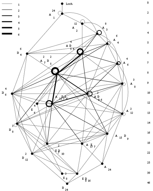
For the chronology below it is perhaps useful to note that, whereas Niemeier’s paper did appear in 1973, it was submitted april 5th 1971 and is just a minor rewrite of Niemeier’s Ph.D. “Definite quadratische Formen der Dimension 24 und Diskriminante 1” obtained in 1968 from the University of Göttingen with advisor Martin Kneser.

The claim

On page 328 of Ernst Witt’s Collected Papers Ina Kersten recalls that Witt gave a colloquium talk on January 27, 1970 in Hamburg entitled “Gitter und Mathieu-Gruppen” (Lattices and Mathieu-groups). In this talk Witt claimed to have found nine lattices in $ {\Gamma_{24}} $ as far back as 1938 and that on January 28, 1940 he found two additional lattices $ {M} $ and $ {\Lambda} $ while studying the Steiner system $ {S(5,8,24)} $.

On page 329 of the collected papers is a scan of the abstract Witt wrote in the colloquium book in Bielefeld where he gave a talk “Uber einige unimodularen Gitter” (On certain unimodular lattices) on January 28, 1972

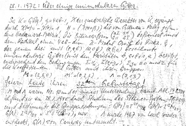
Here, Witt claims that he found three new lattices in $ {\Gamma_{24}} $ on January 28, 1940 as the lattices $ {M} $, $ {M’} $ and $ {\Lambda} $ ‘feiern heute ihren 32sten Gebursttag!’ (celebrate today their 32nd birthday).

He goes on telling that the lattices $ {M} $ and $ {\Lambda} $ were number 10 and 11 in his list of lattices in $ {\Gamma_{24}} $ in his paper “Eine Identität zwischen Modulformen zweiten Grades” in the Abh. Math. Sem. Univ. Hamburg 14 (1941) 323-337 and he refers in particular to page 324 of that paper.

He further claims that he computed the orders of their automorphism groups and writes that $ {\Lambda} $ ‘wurde 1967 von Leech wieder-entdeckt’ (was re-discovered by Leech in 1967) and that its automorphism group $ {G(\Lambda)} $ was studied by John Conway. Recall that Conway’s investigations of the automorphism group of the Leech lattice led to the discovery of three new sporadic groups, the Conway groups $ {Co_1,Co_2} $ and $ {Co_3} $.

However, Witt’s 1941-paper does not contain a numbered list of 24-dimensional lattices. In fact, apart from $ {E_8+E_8+E_8} $ is does not contain a single lattice in $ {\Gamma_{24}} $. The only relevant paragraph is indeed on page 324

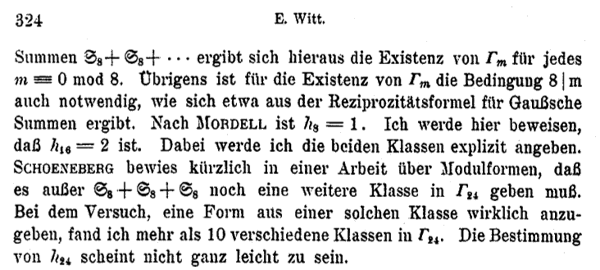
He observes that Mordell already proved that there is just one lattice in $ {\Gamma_8} $ (the $ {E_8} $-lattice) and that the main result of his paper is to prove that there are precisely two even unimodular 16-dimensional lattices : $ {E_8+E_8} $ and another lattice, now usually called the 16-dimensional Witt-lattice.

He then goes on to observe that Schoeneberg knew that $ {\# \Gamma_{24} > 1} $ and so there must be more lattices than $ {E_8+E_8+E_8} $ in $ {\Gamma_{24}} $. Witt concludes with : “In my attempt to find such a lattice, I discovered more than 10 lattices in $ {\Gamma_{24}} $. The determination of $ {\# \Gamma_{24}} $ does not seem to be entirely trivial.”

Hence, it is fair to assume that by 1940 Ernst Witt had discovered at least 11 of the 24 Niemeier lattices. Whether the Leech lattice was indeed lattice 11 on the list is anybody’s guess.

Next time we will look more closely into the historical context of Witt’s 1941 paper.

One Comment

Klein’s dessins d’enfant and the buckyball

Published June 30, 2008 by lievenlb

We saw that the icosahedron can be constructed from the alternating group $A_5 $ by considering the elements of a conjugacy class of order 5 elements as the vertices and edges between two vertices if their product is still in the conjugacy class.

This description is so nice that one would like to have a similar construction for the buckyball. But, the buckyball has 60 vertices, so they surely cannot correspond to the elements of a conjugacy class of $A_5 $. But, perhaps there is a larger group, somewhat naturally containing $A_5 $, having a conjugacy class of 60 elements?

This is precisely the statement contained in Galois’ last letter. He showed that 11 is the largest prime p such that the group $L_2(p)=PSL_2(\mathbb{F}_p) $ has a (transitive) permutation presentation on p elements. For, p=11 the group $L_2(11) $ is of order 660, so it permuting 11 elements means that this set must be of the form $X=L_2(11)/A $ with $A \subset L_2(11) $ a subgroup of 60 elements… and it turns out that $A \simeq A_5 $…

Actually there are TWO conjugacy classes of subgroups isomorphic to $A_5 $ in $L_2(11) $ and we have already seen one description of these using the biplane geometry (one class is the stabilizer subgroup of a ‘line’, the other the stabilizer subgroup of a point).

Here, we will give yet another description of these two classes of $A_5 $ in $L_2(11) $, showing among other things that the theory of dessins d’enfant predates Grothendieck by 100 years.

In the very same paper containing the first depiction of the Dedekind tessellation, Klein found that there should be a degree 11 cover $\mathbb{P}^1_{\mathbb{C}} \rightarrow \mathbb{P}^1_{\mathbb{C}} $ with monodromy group $L_2(11) $, ramified only in the three points ${ 0,1,\infty } $ such that there is just one point lying over $\infty $, seven over 1 of which four points where two sheets come together and finally 5 points lying over 0 of which three where three sheets come together. In 1879 he wanted to determine this cover explicitly in the paper “Ueber die Transformationen elfter Ordnung der elliptischen Funktionen” (Math. Annalen) by describing all Riemann surfaces with this ramification data and pick out those with the correct monodromy group.

He manages to do so by associating to all these covers their ‘dessins d’enfants’ (which he calls Linienzuges), that is the pre-image of the interval [0,1] in which he marks the preimages of 0 by a bullet and those of 1 by a +, such as in the innermost darker graph on the right above. He even has these two wonderful pictures explaining how the dessin determines how the 11 sheets fit together. (More examples of dessins and the correspondences of sheets were drawn in the 1878 paper.)

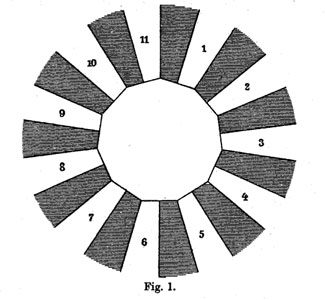
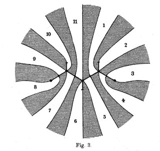
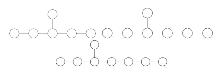
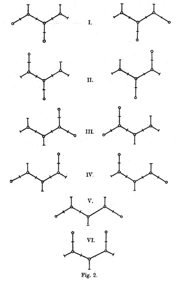
The ramification data translates to the following statements about the Linienzuge : (a) it must be a tree ($\infty $ has one preimage), (b) there are exactly 11 (half)edges (the degree of the cover),
(c) there are 7 +-vertices and 5 o-vertices (preimages of 0 and 1) and (d) there are 3 trivalent o-vertices and 4 bivalent +-vertices (the sheet-information).

Klein finds that there are exactly 10 such dessins and lists them in his Fig. 2 (left). Then, he claims that one the two dessins of type I give the correct monodromy group. Recall that the monodromy group is found by giving each of the half-edges a number from 1 to 11 and looking at the permutation $\tau $ of order two pairing the half-edges adjacent to a +-vertex and the order three permutation $\sigma $ listing the half-edges by cycling counter-clockwise around a o-vertex. The monodromy group is the group generated by these two elements.

Fpr example, if we label the type V-dessin by the numbers of the white regions bordering the half-edges (as in the picture Fig. 3 on the right above) we get
$\sigma = (7,10,9)(5,11,6)(1,4,2) $ and $\tau=(8,9)(7,11)(1,5)(3,4) $.

Nowadays, it is a matter of a few seconds to determine the monodromy group using GAP and we verify that this group is $A_{11} $.

Of course, Klein didn’t have GAP at his disposal, so he had to rule out all these cases by hand.

gap> g:=Group((7,10,9)(5,11,6)(1,4,2),(8,9)(7,11)(1,5)(3,4));
Group([ (1,4,2)(5,11,6)(7,10,9), (1,5)(3,4)(7,11)(8,9) ])
gap> Size(g);
19958400
gap> IsSimpleGroup(g);
true

Klein used the fact that $L_2(11) $ only has elements of orders 1,2,3,5,6 and 11. So, in each of the remaining cases he had to find an element of a different order. For example, in type V he verified that the element $\tau.(\sigma.\tau)^3 $ is equal to the permutation (1,8)(2,10,11,9,6,4,5)(3,7) and consequently is of order 14.

Perhaps Klein knew this but GAP tells us that the monodromy group of all the remaining 8 cases is isomorphic to the alternating group $A_{11} $ and in the two type I cases is indeed $L_2(11) $. Anyway, the two dessins of type I correspond to the two conjugacy classes of subgroups $A_5 $ in the group $L_2(11) $.

But, back to the buckyball! The upshot of all this is that we have the group $L_2(11) $ containing two classes of subgroups isomorphic to $A_5 $ and the larger group $L_2(11) $ does indeed have two conjugacy classes of order 11 elements containing exactly 60 elements (compare this to the two conjugacy classes of order 5 elements in $A_5 $ in the icosahedral construction). Can we construct the buckyball out of such a conjugacy class?

To start, we can identify the 12 pentagons of the buckyball from a conjugacy class C of order 11 elements. If $x \in C $, then so do $x^3,x^4,x^5 $ and $x^9 $, whereas the powers ${ x^2,x^6,x^7,x^8,x^{10} } $ belong to the other conjugacy class. Hence, we can divide our 60 elements in 12 subsets of 5 elements and taking an element x in each of these, the vertices of a pentagon correspond (in order) to $~(x,x^3,x^9,x^5,x^4) $.

Group-theoretically this follows from the fact that the factorgroup of the normalizer of x modulo the centralizer of x is cyclic of order 5 and this group acts naturally on the conjugacy class of x with orbits of size 5.

Finding out how these pentagons fit together using hexagons is a lot subtler… and in The graph of the truncated icosahedron and the last letter of Galois Bertram Kostant shows how to do this.

Fix a subgroup isomorphic to $A_5 $ and let D be the set of all its order 2 elements (recall that they form a full conjugacy class in this $A_5 $ and that there are precisely 15 of them). Now, the startling observation made by Kostant is that for our order 11 element $x $ in C there is a unique element $a \in D $ such that the commutator$~b=[x,a]=x^{-1}a^{-1}xa $ belongs again to D. The unique hexagonal side having vertex x connects it to the element $b.x $which belongs again to C as $b.x=(ax)^{-1}.x.(ax) $.

Concluding, if C is a conjugacy class of order 11 elements in $L_2(11) $, then its 60 elements can be viewed as corresponding to the vertices of the buckyball. Any element $x \in C $ is connected by two pentagonal sides to the elements $x^{3} $ and $x^4 $ and one hexagonal side connecting it to $\tau x = b.x $.

Leave a Comment

Arnold’s trinities

Published June 17, 2008 by lievenlb

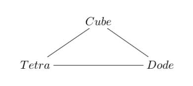
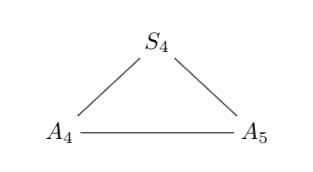
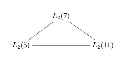
Referring to the triple of exceptional Galois groups $L_2(5),L_2(7),L_2(11) $ and its connection to the Platonic solids I wrote : “It sure seems that surprises often come in triples…”. Briefly I considered replacing triples by trinities, but then, I didnt want to sound too mystic…

David Corfield of the n-category cafe and a dialogue on infinity (and perhaps other blogs I’m unaware of) pointed me to the paper Symplectization, complexification and mathematical trinities by Vladimir I. Arnold. (Update : here is a PDF-conversion of the paper)

The paper is a write-up of the second in a series of three lectures Arnold gave in june 1997 at the meeting in the Fields Institute dedicated to his 60th birthday. The goal of that lecture was to explain some mathematical dreams he had.

The next dream I want to present is an even more fantastic set of theorems and conjectures. Here I also have no theory and actually the ideas form a kind of religion rather than mathematics.
The key observation is that in mathematics one encounters many trinities. I shall present a list of examples. The main dream (or conjecture) is that all these trinities are united by some rectangular “commutative diagrams”.
I mean the existence of some “functorial” constructions connecting different trinities. The knowledge of the existence of these diagrams provides some new conjectures which might turn to be true theorems.

Follows a list of 12 trinities, many taken from Arnold’s field of expertise being differential geometry. I’ll restrict to the more algebraically inclined ones.

1 : “The first trinity everyone knows is”

where $\mathbb{H} $ are the Hamiltonian quaternions. The trinity on the left may be natural to differential geometers who see real and complex and hyper-Kaehler manifolds as distinct but related beasts, but I’m willing to bet that most algebraists would settle for the trinity on the right where $\mathbb{O} $ are the octonions.

2 : The next trinity is that of the exceptional Lie algebras E6, E7 and E8.

with corresponding Dynkin-Coxeter diagrams

Arnold has this to say about the apparent ubiquity of Dynkin diagrams in mathematics.

Manin told me once that the reason why we always encounter this list in many different mathematical classifications is its presence in the hardware of our brain (which is thus unable to discover a more complicated scheme).
I still hope there exists a better reason that once should be discovered.

Amen to that. I’m quite hopeful human evolution will overcome the limitations of Manin’s brain…

3 : Next comes the Platonic trinity of the tetrahedron, cube and dodecahedron

Clearly one can argue against this trinity as follows : a tetrahedron is a bunch of triangles such that there are exactly 3 of them meeting in each vertex, a cube is a bunch of squares, again 3 meeting in every vertex, a dodecahedron is a bunch of pentagons 3 meeting in every vertex… and we can continue the pattern. What should be a bunch a hexagons such that in each vertex exactly 3 of them meet? Well, only one possibility : it must be the hexagonal tiling (on the left below). And in normal Euclidian space we cannot have a bunch of septagons such that three of them meet in every vertex, but in hyperbolic geometry this is still possible and leads to the Klein quartic (on the right). Check out this wonderful post by John Baez for more on this.

4 : The trinity of the rotation symmetry groups of the three Platonics

where $A_n $ is the alternating group on n letters and $S_n $ is the symmetric group.

Clearly, any rotation of a Platonic solid takes vertices to vertices, edges to edges and faces to faces. For the tetrahedron we can easily see the 4 of the group $A_4 $, say the 4 vertices. But what is the 4 of $S_4 $ in the case of a cube? Well, a cube has 4 body-diagonals and they are permuted under the rotational symmetries. The most difficult case is to see the $5 $ of $A_5 $ in the dodecahedron. Well, here’s the solution to this riddle

there are exactly 5 inscribed cubes in a dodecahedron and they are permuted by the rotations in the same way as $A_5 $.

7 : The seventh trinity involves complex polynomials in one variable

the Laurant polynomials and the modular polynomials (that is, rational functions with three poles at 0,1 and $\infty $.

8 : The eight one is another beauty

Here ‘numbers’ are the ordinary complex numbers $\mathbb{C} $, the ‘trigonometric numbers’ are the quantum version of those (aka q-numbers) which is a one-parameter deformation and finally, the ‘elliptic numbers’ are a two-dimensional deformation. If you ever encountered a Sklyanin algebra this will sound familiar.

This trinity is based on a paper of Turaev and Frenkel and I must come back to it some time…

The paper has some other nice trinities (such as those among Whitney, Chern and Pontryagin classes) but as I cannot add anything sensible to it, let us include a few more algebraic trinities. The first one attributed by Arnold to John McKay

13 : A trinity parallel to the exceptional Lie algebra one is

between the 27 straight lines on a cubic surface, the 28 bitangents on a quartic plane curve and the 120 tritangent planes of a canonic sextic curve of genus 4.

14 : The exceptional Galois groups

explained last time.

15 : The associated curves with these groups as symmetry groups (as in the previous post)

where the ? refers to the mysterious genus 70 curve. I’ll check with one of the authors whether there is still an embargo on the content of this paper and if not come back to it in full detail.

16 : The three generations of sporadic groups

Do you have other trinities you’d like to worship?

Leave a Comment

Hexagonal Moonshine (3)

Published July 13, 2007 by lievenlb

Hexagons keep on popping up in the representation theory of the modular group and its close associates. We have seen before that singularities in 2-dimensional representation varieties of the three string braid group $B_3 $ are ‘clanned together’ in hexagons and last time Ive mentioned (in passing) that the representation theory of the modular group is controlled by the double quiver of the extended Dynkin diagram $\tilde{A_5} $, which is an hexagon…

Today we’re off to find representations of the extended modular group $\tilde{\Gamma} = PGL_2(\mathbb{Z}) $, which is obtained by adding to the modular group (see this post for a proof of generation)

$\Gamma = \langle U=\begin{bmatrix} 0 & -1 \\\ 1 & 0 \end{bmatrix},V=\begin{bmatrix} 0 & 1 \\\ -1 & 1 \end{bmatrix} \rangle $ the matrix $R=\begin{bmatrix} 0 & 1 \\\ 1 & 0 \end{bmatrix} $

In terms of generators and relations, one easily verfifies that

$\tilde{\Gamma} = \langle~U,V,R~|~U^2=R^2=V^3=(RU)^2=(RV)^2=1~\rangle $

and therefore $\tilde{\Gamma} $ is the amalgamated free product of the dihedral groups $D_2 $ and $D_3 $ over their common subgroup $C_2 = \langle~R~\rangle $, that is

$\tilde{\Gamma} = \langle U,R | U^2=R^2=(RU)^2=1 \rangle \ast_{\langle R | R^2=1 \rangle} \langle V,R | V^3=R^2=(RV)^2=1 \rangle = D_2 \ast_{C_2} D_3 $

From this description it is easy to find all n-dimensional $\tilde{\Gamma} $-representations $V $ and relate them to quiver-representations. $D_2 = C_2 \times C_2 $ and hence has 4 1-dimensonal simples $S_1,S_2,S_3,S_4 $. Restricting $V\downarrow_{D_2} $ to the subgroup $D_2 $ it decomposes as

$V \downarrow_{D_2} \simeq S_1^{\oplus a_1} \oplus S_2^{\oplus a_2} \oplus S_3^{\oplus a_3} \oplus S_4^{\oplus a_4} $ with $a_1+a_2+a_3+a_4=n $

Similarly, because $D_3=S_3 $ has two one-dimensional representations $T,S $ (the trivial and the sign representation) and one simple 2-dimensional representation $W $, restricting $V $ to this subgroup gives a decomposition

$V \downarrow_{D_3} \simeq T^{b_1} \oplus S^{\oplus b_2} \oplus W^{\oplus b_3} $, this time with $b_1+b_2+2b_3=n $

Restricting both decompositions further down to the common subgroup $C_2 $ one obtains a $C_2 $-isomorphism $V \downarrow_{D_2} \rightarrow^{\phi} V \downarrow_{D_3} $ which implies also that the above numbers must be chosen such that $a_1+a_3=b_1+b_3 $ and $a_2+a_4=b_2+b_3 $. We can summarize all this info about $V $ in a representation of the quiver

Here, the vertex spaces on the left are the iso-typical factors of $V \downarrow_{D_2} $ and those on the right those of $V \downarrow_{D_3} $ and the arrows give the block-components of the $C_2 $-isomorphism $\phi $. The nice things is that one can also reverse this process to get all $\tilde{\Gamma} $-representations from $\theta $-semistable representations of this quiver (having the additional condition that the square matrix made of the arrows is invertible) and isomorphisms of group-representation correspond to those of quiver-representations!

This proves that for all n the varieties of n-dimensional representations $\mathbf{rep}_n~\tilde{\Gamma} $ are smooth (but have several components corresponding to the different dimension vectors $~(a_1,a_2,a_3,a_4;b_1,b_2,b_3) $ such that $\sum a_i = n = b_1+b_2+2b_3 $.

The basic principle of _M-geometry_ is that a lot of the representation theory follows from the ‘clan’ (see this post) determined by the simples of smallest dimensions. In the case of the extended modular group $\tilde{\Gamma} $ it follows that there are exactly 4 one-dimensional simples and exactly 4 2-dimensional simples, corresponding to the dimension vectors

$\begin{cases} a=(0,0,0,1;0,1,0) \\\ b=(0,1,0,0;0,1,0) \\\ c=(1,0,0,0;1,0,0) \\\ d=(0,0,1,0;1,0,0) \end{cases} $ resp. $\begin{cases} e=(0,1,1,0;0,0,1) \\\ f=(1,0,0,1;0,0,1) \\\ g=(0,0,1,1;0,0,1) \\\ h=(1,1,0,0;0,0,1) \end{cases} $

If one calculates the ‘clan’ of these 8 simples one obtains the double quiver of the graph on the left. Note that a and b appear twice, so one should glue the left and right hand sides together as a Moebius-strip. That is, the clan determining the representation theory of the extended modular group is a Moebius strip made of two hexagons!

However, one should not focuss too much on the hexagons (that is, the extended Dynkin diagram $\tilde{A_5} $) here. The two ‘backbones’ (e–f and g–h) have their vertices corresponding to 2-dimensional simples whereas the topand bottom vertices correspond to one-dimensional simples. Hence, the correct way to look at this clan is as two copies of the double quiver of the extended Dynkin diagram $\tilde{D_5} $ glued over their leaf vertices to form a Moebius strip. Remark that the components of the sotropic root of $\tilde{D_5} $ give the dimensions of the corresponding $\tilde{\Gamma} $ simples.

The remarkable ubiquity of (extended) Dynkins never ceases to amaze!

One Comment

Hexagonal Moonshine (2)

Published July 11, 2007 by lievenlb

Delving into finite dimensional representations of the modular group $\Gamma = PSL_2(\mathbb{Z}) $ it is perhaps not too surprising to discover numerical connections with modular functions. Here, one such strange observation and a possible explanation.

Using the _fact_ that the modular group $\Gamma = PSL_2(\mathbb{Z}) $ is the free group product $C_2 \ast C_3 $ it is fairly easy to see that the variety of all n-dimensional representations $\mathbf{rep}_n~\Gamma $ is smooth (though it contains several connected components). Some of these components will contain simple representations, some will not. Anyway, we are not interested in all n-dimensional representations but in the isomorphism classes of such representations. The best algebraic approximation to this problem is by studying the quotient varieties

$\mathbf{iss}_n~\Gamma = \mathbf{rep}_n~\Gamma // GL(n) $

under the action of $GL(n) $ by basechange. Geometric invariant theory tells us that the points of this quotient variety correspond to isoclasses of semi-simple n-dimensional representations (whence the notation $\mathbf{iss}_n $). Again, these quotient varieties split into several connected components, some of which will have an open subset of points corresponding to simple representations.

It is a natural idea to compute the codimension of subvariety of proper semi-simples in the component of maximal dimension containing simple representations. _M-geometry_ allows you to reduce such calculation to quiver-problems. Anyway, if one does this for small values of n one obtains the following sequence of codimension-numbers (starting with $n=1 $

0,1,1,1,1,3,1,3,3,3,3,5,3,5,5,5,5,7,5,7,…

which doesnt seem too exciting before you feed it to Sloan’s integer sequences encyclopedia when one discovers that it is precisely sequence A063195 which gives the dimensions of weight 2n _cuspidal newforms_
for $\Gamma_0(6) $…

The optimistic “moonshine”-interpretation of this might be that these newforms can be viewed somehow as functions on the varieties of finite dimensional $\Gamma $-representations having the property that they pick out generic simple representations as their non-zeroes.

Be that as it may (one never knows in these matters), here a more down-to-earth explanation. The sequence A063195 obviously has a 6-periodicity behaviour so it suffices to understand why the codimension-sequence should have a similar feature (modulo computing the first few terms of it and observing the coincidence with the first few terms of A063195).

The modular group has exactly 6 one-dimensional representations and if one calculates their clan as in hexagonal moonshine (1) one obtains the hexagonal quiver

[tex]\xymatrix{& \vtx{S_1} \ar@/^/[dl] \ar@/^/[dr] & \\ \vtx{S_6} \ar@/^/[ur] \ar@/^/[d] & & \vtx{S_2} \ar@/^/[ul] \ar@/^/[d] \\ \vtx{S_5} \ar@/^/[u] \ar@/^/[dr] & & \vtx{S_3} \ar@/^/[u] \ar@/^/[dl] \\ & \vtx{S_4} \ar@/^/[ur] \ar@/^/[ul] & }[/tex]

M-geometry tells us that this clan contains enough information to determine the components of $\mathbf{rep}_n~\Gamma $ that contain simple representations. They correspond to dimension-vectors of this hexagonal quiver, say

$~(a_1,a_2,a_3,a_4,a_5,a_6) $

such that $a_i \leq a_{i-1}+a_{i+1} $. Moreover, the component is of maximal dimension if the components $a_i $ are evenly spread over the six vertices.
This then explains that the codimension sequence we are interested in must satisfy 6-periodicity.

Reference

This post corrects the erroneous statement made in math.AG/0610587 that the codimension sequence are the dimensions of weight 2n modular forms. The day the paper hit the arXiv I informed the author of the mistakes he made and told him how they could be corrected. Having waited 9 months I’ve given up hope that a revision/correction is imminent.

Leave a Comment

Hexagonal Moonshine (1)

Published June 18, 2007 by lievenlb

Over at the Arcadian Functor, Kea is continuing her series of blog posts on M-theory (the M is supposed to mean either Monad or Motif). A recurrent motif in them is the hexagon and now I notice hexagons popping up everywhere. I will explain some of these observations here in detail, hoping that someone, more in tune with recent technology, may have a use for them.

The three string braid group $B_3 $ is expected to play a crucial role in understanding monstrous moonshine so we should know more about it, for example about its finite dimensional representations. Now, _M geometry_ is pretty good at classifying finite dimensional representations provided the algebra is “smooth” which imples that for every natural number n the variety $\mathbf{rep}_n~A $ of n-dimensional representations of A is a manifold. Unfortunately, the group algebra $A=\mathbb{C} B_3 $ of the three string braid group is singular as we will see in a moment and the hunt for singularities in low dimensional representation varieties will reveal hexagons.

One Comment

football representation theory

Published June 9, 2006 by lievenlb

Unless
you never touched a football in your life (that’s a _soccer-ball_
for those of you with an edu account) you will know that the world
championship in Germany starts tonight. In the wake of it, the field of
‘football-science’ is booming. The BBC runs its The
Science of Football-site and did you know the following?

Research indicates that watching such a phenomenon is not
only exciting, it can be good for our health too. The Scottish
researchers found that there were 14% fewer psychiatric admissions in
the weeks after one World Cup than before it started.

But, would you believe that some of the best people in the field
(Kostant and Sternberg to name a few) have written papers on the
representation theory of a football? Perhaps this becomes more plausible
when you realize that a football has the same shape as the buckyball aka Carbon60.
Because the football (or buckyball) is a truncated icosahedron, its
symmetry group is $A_5$, the smallest of all simple groups and its
representations explain some physical properties of the buckyball. Some
of these papers are freely available and are an excellent read. In fact,
I’m thinking of using them in my course on representations of finite
groups, nxt year. Mathematics and the Buckyball by Fan
Chung and Schlomo Sternberg is a marvelous introduction to
representation theory. Among other things they explain how Schur’s
lemma, Frobenius reciprocity and Maschke’s theorem are used to count the
number of lines in the infra red buckyball spectrum! The Graph of the
Truncated Icosahedron and the Last Letter of Galois by Bertram
Kostant explains the observation, first made by Galois in his last
letter to Chevalier, that $A_{5} = PSL_2(\mathbb{F}_5)$ embeds into
$PSL_{2}(\mathbb{F}_{11})$ and applies this to the buckyball.

In effect, the model we are proposing for C60is such that
each carbon atom can be labeled by an element of order 11 in PSl(2,11)
in such a fashion that the carbon bonds can be expressed in terms of the
group structure of PSl(2,11). It will be seen that the twelve pentagons
are exactly the intersections of M with the twelve Borel sub- groups of
PSl(2,11). (A Borel subgroup is any subgroup which is conjugate to the
group PSl(2,11) defined in (2).) In particular the pentagons are the
maximal sets of commuting elements in M. The most subtle point is the
natural existence of the hexagonal bonds. This will arise from a group
theoretic linkage of any element of order 11 in one Borel subgroup with
a uniquely defined element of order 11 in another Borel subgroup.

These authors consequently joined forces to write Groups and the
Buckyball in which they give further applications of the Galois
embeddings to the electronic spectrum of the buckyball. Another
account can be found in the Master Thesis by Joris Mooij called The
vibrational spectrum of Buckminsterfullerene – An application of
symmetry reduction and computer algebra. Plenty to read should
tonight’s match Germany-Costa Rica turn out to be boring…

Leave a Comment

dvonn (1) mobility

Published January 7, 2006 by lievenlb

[Dvonn](http://www.gipf.com/dvonn $ is
the fourth game in the [Gipf Project](http://www.gipf.com/project_gipf/index.html) and the most
mathematical of all six. It is a very fast (but subtle) game with a
simple [set of rules](http://www.gipf.com/dvonn/rules/rules.html). Here
is a short version

DVONN is a stacking game. It is played
on an elongated hexagonal board, with 23 white, 23 black and 3 red
DVONN-pieces. In the beginning the board is empty. The players first
place the DVONN-pieces on the board and next their own pieces. Then they
start stacking pieces on top of each other. A single piece may be moved
1 space in any direction, a stack of two pieces may be moved two spaces,
etc. A stack must always be moved as a whole and a move must always end
on top of another piece or stack. If pieces or stacks lose contact with
the DVONN pieces, they must be removed from the board. The game ends
when no more moves can be made. The players put the stacks they control
on top of each other and the one with the highest stack is the winner.
That’s all!

All this will become clearer once we fix a
specific end-game, for example

$\xymatrix@=.3cm @!C @R=.7cm{ & &
\Black{2} \connS & & \bull{d}{5} \conn & & \bull{e}{5} \conn & &
\bull{f}{5} \conn & & \bull{g}{5} \conn & & \bull{h}{5} \conn & &
\SWhite \connS & & \SWhite \connS & & \SWhite \conneS & & \\ &
\bull{b}{4} \conn & & \SBlack \connS & & \Black{6} \connS & &
\bull{e}{4} \conn& & \bull{f}{4} \conn & & \bull{g}{4} \conn & &
\bull{h}{4} \conn & & \SWhite \connS & & \SWhite \connS & & \SWhite
\conneS & \\ \SBlack \connbeginS & & \SBlack \connS & & \BDvonn{7}
\connS & & \bull{d}{3} \conn & & \SBlack \connS & & \BDvonn{6} \connS &
& \bull{g}{3} \conn & & \bull{h}{3} \conn & & \Dvonn \connS & & \SWhite
\connS & & \SWhite \connendS \\ & \Black{5} \connbeginS & &
\bull{b}{2} \conn & & \SBlack \connS & & \bull{d}{2} \conn & &
\bull{e}{2} \conn & & \bull{f}{2} \conn & & \bull{g}{2} \conn & &
\bull{h}{2} \conn & & \SWhite \connS & & \SWhite \connendS & \\ & &
\bull{a}{1} \con & & \bull{b}{1} \con & & \Black{5} \conS & &
\bull{d}{1} \con & & \bull{e}{1} \con & & \bull{f}{1} \con & &
\bull{g}{1} \con & & \bull{h}{1} \con & & \White{2} & &} $

with
White to move. Some comments about notation : the left-slanted columns
are denoted by letters from a (left) to k (right) and the rows are
labeled 1 to 5 from bottom to top (surprisingly this ‘standard’
webgame-notation differs from the numbering on my Dvonn-board where the
rows are labeled from top to bottom…). So, for example, the three
spots on the upper right are k3,k4 and k5 (there are no k1 or k2 spots).
The three Dvonn pieces are colored red and in the course of the game a
stack may land on a Dvonn piece and so stacks containing a Dvonn piece
are denoted with a red halo. For example, the symbol on spot f3 stands
for for a stack of 6 pieces, one of which is a red Dvonn piece, under
the control of Black (that is, the top-piece is Black). Further note
that a piece or stack can only move if it is not surrounded by 6 other
pieces or stacks (so the White pieces on j3 and j4 cannot (yet) move). A
piece can only move by one step in either line-direction provided there
is another piece or stack on that position. The same applies for stacks
: an height 3 stack for example can move in each lin-direction by
exactly 3 steps provided there is a piece or stack to jump onto. For
example, the height 6 stack on d4 can only move to j4 whereas the height
6 stack on f3 cannot move at all! Similarly, the two black height 5
stacks are immobile. At the moment black has all its stacks defended,
that is, if White should be able to jump onto one of them (which White
cannot at the moment), Black can use one of its neighbouring pieces to
take the stack back under its control. So, any computer program would
‘evaluate’ the position as favourable for Black : Black has stacks of
total height 34 safely under control (there are no immediate threats to
be seen : the [horizon effect](http://www.comp.lancs.ac.uk/computing/research/aai-aied/people/paulb/old243prolog/subsection3_7_5.html) in such programs) whereas White
can only claim potential stacks of total height 13… Still, Black
has already lost the game. White has more pieces which are quite mobile
as opposed to the immobile black stacks, so Black will soon run out of
moves to make and his end position will have some large stacks on the
third row. All white has to do is to let Black run out of moves and then
continue (Dvonn forces each player to make a move if they still can and
to pass the move otherwise, so the most mobile player can still continue
long after the other player was forced to stop) to build a White stack
of the appropriate height on the third row to jump on the highest Black
stack with its last move! Here is how the play continued : 1) j2-k3 ;
a3-b3 2) i1-k3 ; c5-c3 3) i2-i3 ; c2-c3 4) i3-k3 ; d4-j4 5)
j3-j4 ; e3-f3 6) i4-j4 ; c4-b3 to arrive at the position where
Black is no longer able to make any moves at all

$\xymatrix@=.3cm
@!C @R=.7cm{ & & \bull{c}{5} \conn & & \bull{d}{5} \conn & & \bull{e}{5}
\conn & & \bull{f}{5} \conn & & \bull{g}{5} \conn & & \bull{h}{5} \conn
& & \SWhite \connS & & \SWhite \connS & & \SWhite \conneS & & \\ &
\bull{b}{4} \conn & & \bull{c}{4} \conn & & \bull{d}{4} \conn & &
\bull{e}{4} \conn& & \bull{f}{4} \conn & & \bull{g}{4} \conn & &
\bull{h}{4} \conn & & \bull{i}{4} \connS & & \White{9} \connS & &
\SWhite \conneS & \\ \bull{a}{3} \connbegin & & \Black{3} \connS & &
\BDvonn{10} \connS & & \bull{d}{3} \conn & & \bull{e}{3} \conn & &
\BDvonn{7} \connS & & \bull{g}{3} \conn & & \bull{h}{3} \conn & &
\bull{i}{3} \conn & & \bull{j}{3} \conn & & \WDvonn{6} \connendS \\ &
\Black{5} \connbeginS & & \bull{b}{2} \conn & & \bull{c}{2} \conn & &
\bull{d}{2} \conn & & \bull{e}{2} \conn & & \bull{f}{2} \conn & &
\bull{g}{2} \conn & & \bull{h}{2} \conn & & \bull{i}{2} \conn & &
\bull{j}{2} \connend & \\ & & \bull{a}{1} \con & & \bull{b}{1} \con & &
\bull{c}{1} \con & & \bull{d}{1} \con & & \bull{e}{1} \con & &
\bull{f}{1} \con & & \bull{g}{1} \con & & \bull{h}{1} \con & &
\bull{i}{1} & &} $

Note that all pieces and stacks no longer
connected to a Dvonn piece must be removed. So, for example, after the
third move by Black, the Black height 5 stacks on c1 was removed. All
white now has to do is to built an height 8 stack on k3 and jump onto
the height 10 Black stack on c3 to win the game. The (only) way to do
this is by 7. j5-k5 and 8. k5-k3 to finish with 9. k3-c3 with final
position (note again that the White right-hand pieces and stacks are no
longer connected to a Dvonn piece and are hence removed)

$\xymatrix@=.3cm @!C @R=.7cm{ & & \bull{c}{5} \conn & & \bull{d}{5}
\conn & & \bull{e}{5} \conn & & \bull{f}{5} \conn & & \bull{g}{5} \conn
& & \bull{h}{5} \conn & & \bull{i}{5} \conn & & \bull{j}{5} \conn & &
\bull{k}{5} \conne & & \\\ & \bull{b}{4} \conn & & \bull{c}{4} \conn &
& \bull{d}{4} \conn & & \bull{e}{4} \conn& & \bull{f}{4} \conn & &
\bull{g}{4} \conn & & \bull{h}{4} \conn & & \bull{i}{4} \conn & &
\bull{j}{4} \conn & & \bull{k}{4} \conne & \\\ \bull{a}{3} \connbegin
& & \Black{3} \connS & & \WDvonn{18} \connS & & \bull{d}{3} \conn & &
\bull{e}{3} \conn & & \BDvonn{7} \connS & & \bull{g}{3} \conn & &
\bull{h}{3} \conn & & \bull{i}{3} \conn & & \bull{j}{3} \conn & &
\bull{k}{3} \connend \\\ & \Black{5} \connbeginS & & \bull{b}{2} \conn
& & \bull{c}{2} \conn & & \bull{d}{2} \conn & & \bull{e}{2} \conn & &
\bull{f}{2} \conn & & \bull{g}{2} \conn & & \bull{h}{2} \conn & &
\bull{i}{2} \conn & & \bull{j}{2} \connend & \\\ & & \bull{a}{1} \con &
& \bull{b}{1} \con & & \bull{c}{1} \con & & \bull{d}{1} \con & &
\bull{e}{1} \con & & \bull{f}{1} \con & & \bull{g}{1} \con & &
\bull{h}{1} \con & & \bull{i}{1} & & } $

So White wins with 18 to
Black’s 15. This shows that it is important to maintain mobility and
also that it is possible to win a Dvonn-game from computers. In fact,
the above end-game was played against a computer-program (Black). The
entire game can be found
[here](http://www.littlegolem.net/jsp/game/game.jsp?gid=426457&nmove=91)
.

One Comment