Tag: groups

Who discovered the Leech lattice?

Published November 30, 2010 by lievenlb

The Leech lattice was, according to wikipedia, ‘originally discovered by Ernst Witt in 1940, but he did not publish his discovery’ and it ‘was later re-discovered in 1965 by John Leech’. However, there is very little evidence to support this claim.

The facts

What is certain is that John Leech discovered in 1965 an amazingly dense 24-dimensional lattice $ {\Lambda} $ having the property that unit balls around the lattice points touch, each one of them having exactly 196560 neighbors. The paper ‘Notes on sphere packings’ appeared in 1967 in the Canad. J. Math. 19, 251-267.

Compare this to the optimal method to place pennies on a table, leading to the hexagonal tiling, each penny touching exactly 6 others. Similarly, in dimension 8 the densest packing is the E8 lattice in which every unit ball has exactly 240 neighbors.

The Leech lattice $ {\Lambda} $ can be characterized as the unique unimodular positive definite even lattice such that the length of any non-zero vector is at least two.

The list of all positive definite even unimodular lattices, $ {\Gamma_{24}} $, in dimension 24 was classified later by Hans-Volker Niemeier and are now known as the 24 Niemeier lattices.

For the chronology below it is perhaps useful to note that, whereas Niemeier’s paper did appear in 1973, it was submitted april 5th 1971 and is just a minor rewrite of Niemeier’s Ph.D. “Definite quadratische Formen der Dimension 24 und Diskriminante 1” obtained in 1968 from the University of Göttingen with advisor Martin Kneser.

The claim

On page 328 of Ernst Witt’s Collected Papers Ina Kersten recalls that Witt gave a colloquium talk on January 27, 1970 in Hamburg entitled “Gitter und Mathieu-Gruppen” (Lattices and Mathieu-groups). In this talk Witt claimed to have found nine lattices in $ {\Gamma_{24}} $ as far back as 1938 and that on January 28, 1940 he found two additional lattices $ {M} $ and $ {\Lambda} $ while studying the Steiner system $ {S(5,8,24)} $.

On page 329 of the collected papers is a scan of the abstract Witt wrote in the colloquium book in Bielefeld where he gave a talk “Uber einige unimodularen Gitter” (On certain unimodular lattices) on January 28, 1972

Here, Witt claims that he found three new lattices in $ {\Gamma_{24}} $ on January 28, 1940 as the lattices $ {M} $, $ {M’} $ and $ {\Lambda} $ ‘feiern heute ihren 32sten Gebursttag!’ (celebrate today their 32nd birthday).

He goes on telling that the lattices $ {M} $ and $ {\Lambda} $ were number 10 and 11 in his list of lattices in $ {\Gamma_{24}} $ in his paper “Eine Identität zwischen Modulformen zweiten Grades” in the Abh. Math. Sem. Univ. Hamburg 14 (1941) 323-337 and he refers in particular to page 324 of that paper.

He further claims that he computed the orders of their automorphism groups and writes that $ {\Lambda} $ ‘wurde 1967 von Leech wieder-entdeckt’ (was re-discovered by Leech in 1967) and that its automorphism group $ {G(\Lambda)} $ was studied by John Conway. Recall that Conway’s investigations of the automorphism group of the Leech lattice led to the discovery of three new sporadic groups, the Conway groups $ {Co_1,Co_2} $ and $ {Co_3} $.

However, Witt’s 1941-paper does not contain a numbered list of 24-dimensional lattices. In fact, apart from $ {E_8+E_8+E_8} $ is does not contain a single lattice in $ {\Gamma_{24}} $. The only relevant paragraph is indeed on page 324

He observes that Mordell already proved that there is just one lattice in $ {\Gamma_8} $ (the $ {E_8} $-lattice) and that the main result of his paper is to prove that there are precisely two even unimodular 16-dimensional lattices : $ {E_8+E_8} $ and another lattice, now usually called the 16-dimensional Witt-lattice.

He then goes on to observe that Schoeneberg knew that $ {\# \Gamma_{24} > 1} $ and so there must be more lattices than $ {E_8+E_8+E_8} $ in $ {\Gamma_{24}} $. Witt concludes with : “In my attempt to find such a lattice, I discovered more than 10 lattices in $ {\Gamma_{24}} $. The determination of $ {\# \Gamma_{24}} $ does not seem to be entirely trivial.”

Hence, it is fair to assume that by 1940 Ernst Witt had discovered at least 11 of the 24 Niemeier lattices. Whether the Leech lattice was indeed lattice 11 on the list is anybody’s guess.

Next time we will look more closely into the historical context of Witt’s 1941 paper.

One Comment

Seriously now, where was the Bourbaki wedding?

Published November 25, 2009 by lievenlb

A few days before Halloween, Norbert Dufourcq (who died december 17th 1990…), sent me a comment, containing lots of useful information, hinting I did get it wrong about the church of the Bourbali wedding in the previous post.

Norbert Dufourcq, an organist and student of Andre Machall, the organist-in-charge at the Saint-Germain-des-Prés church in 1939, the place where I speculated the Bourbaki wedding took place, concluded his comment with :

“P.S. Lieven, you _do_ know about the Schola Cantorum, now, don’t you?!?”.

Euh… actually … no, I did not …

La Schola Cantorum is a private music school in Paris. It was founded in 1894 by Charles Bordes, Alexandre Guilmant and Vincent d’Indy as a counterbalance to the Paris Conservatoire’s emphasis on opera. Its alumni include many significant figures in 20th century music, such as Erik Satie and Cole Porter.

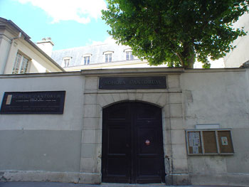
Schola Cantorum is situated 69, rue Saint Jacques, Paris, just around the corner of the Ecole Normal Superieure, home base to the Bourbakis. In fact, closer investigation reveals striking similarities and very close connections between the circle of artists at la Schola and the Bourbaki group.

In december 1934, the exact month the Bourbaki group was formed, a radical reorganisation took place at the Schola, when Nestor Lejeune became the new director. He invited several young musicians, many from the famous Dukas-class, to take up teaching positions at the Schola.

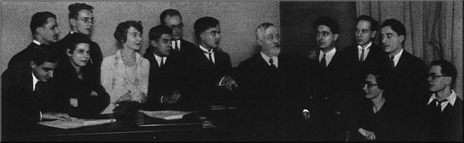
Here’s a picture of part of the Dukas class of 1929, several of its members will play a role in the upcoming events :
from left to right next to the piano : Pierre Maillard-Verger, Elsa Barraine, Yvonne Desportes, Tony Aubin, Pierre Revel, Georges Favre, Paul Dukas, René Duclos, Georges Hugon, Maurice Duruflé. Seated on the right : Claude Arrieu, Olivier Messiaen.

The mid-1930s in Paris saw the emergence of two closely-related groups with a membership which overlapped : La Spirale and La Jeune France. La Spirale was founded in 1935 under the leadership of Georges Migot; its other committee members were Paul Le Flem, his pupil André Jolivet, Edouard Sciortino, Claire Delbos, her husband Olivier Messiaen, Daniel-Lesur and Jules Le Febvre. The common link between almost all of these musicians was their connection with the Schola Cantorum.

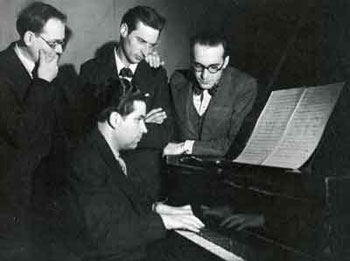On the left : Les Jeunes Musiciens Français : André Jolivet on the Piano. Standing from left to right :
Olivier Messiaen, Yves Baudrier, Daniel-Lesur.

Nigel Simeone wrote this about Messiaen and La Jeune France :
“The extremely original and independent-minded Messiaen had already shown himself to be a rather unexpected enthusiast for joining groups: in December 1932 he wrote to his friend Claude Arrieu about a letter from another musician, Jacques Porte, outlining plans for a new society to be called Les Jeunes Musiciens Français.
Messiaen agreed to become its vice-president, but nothing seems to have come of the project. Six months later, in June 1933, he had a frustrating meeting with Roger Désormière on behalf of the composers he described to Arrieu as ‘les quatre’, all of them Dukas pupils: Elsa Barraine, the recently-deceased Jean Cartan, Arrieu and Messiaen himself; during the early 1930s Messiaen and Arrieu organised concerts featuring all four composers.”

Finally, we’re getting a connection with the Bourbaki group! Norbert Dufourcq mentioned it already in his comment “Messiaen was also a good friend of Jean Cartan (himself a composer, and Henri’s brother)”. Henri Cartan was one of the first Bourbakis and an excellent piano player himself.

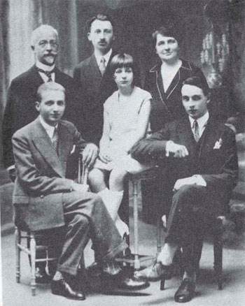
The Cartan family picture on the right : standing from left to right, father Elie Cartan (one of the few older French mathematicians respected by the Bourbakis), Henri and his mother Marie-Louise. Seated, the younger children, from left to right : Louis, Helene (who later became a mathematician, herself) and the composer Jean Cartan, who sadly died very young from tuberculoses in 1932…

The december 1934 revolution in French music at the Schola Cantorum, instigated by Messiaen and followers, was the culmination of a process that started a few years before when Jean Cartan was among the circle of revolutionados. Because Messiaen was a fiend of the Cartan family, they surely must have been aware of the events at the Schola (or because it was merely a block away from the ENS), and, the musicians’ revolt may very well have been an example to follow for the first Bourbakis…(?!)

Anyway, we now know the intended meaning of the line “with lemmas sung by the Scholia Cartanorum” on the wedding-invitation. Cartanorum is NOT (as I claimed last time) bad Latin for ‘Cartesiorum’, leading to Descartes and the Saint-Germain-des-Pres church, but is in fact passable Latin (plur. gen.) of CARTAN(us), whence the translation “with lemmas sung by the school of the Cartans”. There’s possibly a double pun intended here : first, a reference to (father) Cartan’s lemma and, of course, to La Schola where the musical Cartan-family felt at home.

Fine, but does this brings us any closer to the intended place of the Bourbaki-Petard wedding? Well, let’s reconsider the hidden ‘clues’ we discovered last time : the phrase “They will receive the trivial isomorphism from P. Adic, of the Order of the Diophantines” might suggest that the church belongs to a a religious order and is perhaps an abbey- or convent-church and the phrase “the organ will be played by Monsieur Modulo” requires us to identify this mysterious Mister Modulo, because Norbert Dufourcq rightfully observed :

“note however that in 1939, it wasn’t as common to have a friend-organist perform at a wedding as it is today: the appointed organists, especially at prestigious Paris positions, were much less likely to accept someone play in their stead.”

The history of La Schola Cantorum reveals something that might have amused Frank Smithies (remember he was one of the wedding-invitation-composers) : the Schola is located in the Convent(!) of the Brittish Benedictines…

In 1640 some Benedictine monks, on the run after the religious schism in Britain, found safety in Paris under the protection of Cardinal Richelieu and Anne of Austria at Val-de-Grace, where the Schola is now housed.

As is the case with most convents, the convent of the Brittish Benedictines did have its own convent church, now called l’église royale Notre-Dame du Val-de-Grâce (remember that one of the possible interpretations for “of the universal variety” was that the name of the church would be “Notre-Dame”…).

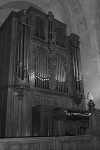This church is presently used as the concert hall of La Schola and is famous for its … musical organ : “In 1853, Aristide Cavaillé-Coll installed a new organ in the Church of Sainte-geneviève which had been restored in its rôle as a place of worship by Prince President Louis-Napoléon. In 1885, upon the decision of President Jules Grévy, this church once again became the Pantheon and, six years later, according to an understanding between the War and Public Works Departments, the organ was transferred to the Val-de-Grâce, under the supervision of the organ builder Merklin. Beforehand, the last time it was heard in the Pantheon must have been for the funeral service of Victor Hugo.
In 1927, a raising was carried out by the builder Paul-Marie Koenig, and the inaugural concert was given by André Marchal and Achille Philippe, the church’s organist. Added to the register of historic monument in 1979, Val-de-Grâce’s “ little great organ ”, as Cavaillé-Coll called it, was restored in 1993 by the organ builders François Delangue and Bernard Hurvy.
The organ of Val-de-Grâce is one the rare parisian surviving witnesses of the art of Aristide Cavaillé-Coll, an instrument that escaped abusive and definitive transformations or modernizations. This explain why, in spite of its relatively modest scale, this organ enjoys quite a reputation, and this, as far as the United States.”

By why would the Val-de-Grace organiste at the time Achille Philip, “organiste titulaire du Val-de-Grâce de 1903 à 1950 et professeur d’orgue et d’harmonie à la Schola Cantorum de 1904 à 1950”, be called ‘Mister Modulo’ in the wedding-invitations line “L’orgue sera tenu par Monsieur Modulo”???

Again, the late Norbert Dufourcq comes to our rescue, proposing a good candidate for ‘Monsieur Modulo’ : “As for “modulo”, note that the organist at Notre-Dame at that time, Léonce de Saint-Martin, was also the composer of a “Suite Cyclique”, though I admit that this is just wordplay: there is nothing “modular” about this work. Maybe a more serious candidate would be Olivier Messiaen (who was organist at the Église de la Trinité): his “modes à transposition limitée” are really about Z/12Z→Z/3Z and Z/12Z→Z/4Z. “

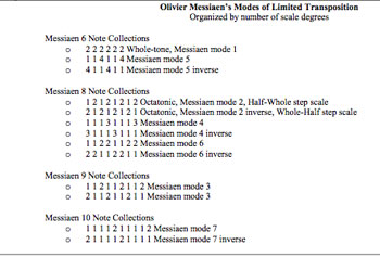Messiaen’s ‘Modes of limited transposition’ were compiled in his book ‘Technique de mon langage musical’. This book was published in Paris by Leduc, as late as 1944, 5 years after the wedding-invitation.

Still, several earlier works of Messiaen used these schemes, most notably La Nativité du Seigneur, composed in 1935 : “The work is one of the earliest to feature elements that were to become key to Messiaen’s later compositions, such as the extensive use of the composer’s own modes of limited transposition, as well as influence from birdsong, and the meters and rhythms of Ancient Greek and traditional Indian music.”

More details on Messiaen’s modes and their connection to modular arithmetic can be found in the study Implementing Modality in Algorithmic Composition by Vincent Joseph Manzo.

Hence, Messiaen is a suitable candidate for the title ‘Monsieur Modulo’, but would he be able to play the Val-de-Grace organ while not being the resident organist?

Remember, the Val-de-Grace church was the concert hall of La Schola, and its musical organ the instrument of choice for the relevant courses. Now … Olivier Messiaen taught at the Schola Cantorum and the École Normale de Musique from 1936 till 1939. So, at the time of the Bourbaki-Petard wedding he would certainly be allowed to play the Cavaillé-Coll organ.

Perhaps we got it right, the second time around : the Bourbaki-Pétard wedding was held on June 3rd 1939 in the church ‘l’église royale Notre-Dame du Val-de-Grâce’ at 12h?

3 Comments

Conway’s big picture

Published May 2, 2009 by lievenlb

Conway and Norton showed that there are exactly 171 moonshine functions and associated two arithmetic subgroups to them. We want a tool to describe these and here’s where Conway’s big picture comes in very handy. All moonshine groups are arithmetic groups, that is, they are commensurable with the modular group. Conway’s idea is to view several of these groups as point- or set-wise stabilizer subgroups of finite sets of (projective) commensurable 2-dimensional lattices.

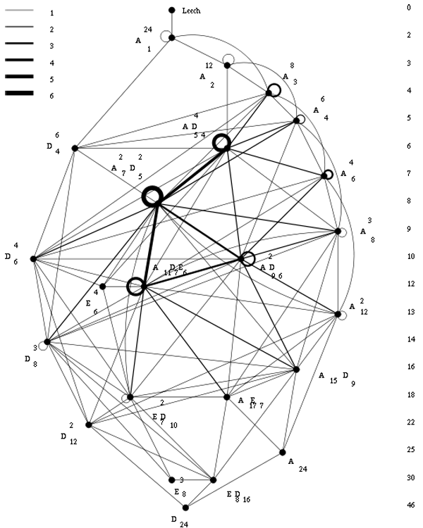
Expanding (and partially explaining) the original moonshine observation of McKay and Thompson, John Conway and Simon Norton formulated monstrous moonshine :

To every cyclic subgroup $\langle m \rangle $ of the Monster $\mathbb{M} $ is associated a function

$f_m(\tau)=\frac{1}{q}+a_1q+a_2q^2+\ldots $ with $q=e^{2 \pi i \tau} $ and all coefficients $a_i \in \mathbb{Z} $ are characters at $m $ of a representation of $\mathbb{M} $. These representations are the homogeneous components of the so called Moonshine module.

Each $f_m $ is a principal modulus for a certain genus zero congruence group commensurable with the modular group $\Gamma = PSL_2(\mathbb{Z}) $. These groups are called the moonshine groups.

Conway and Norton showed that there are exactly 171 different functions $f_m $ and associated two arithmetic subgroups $F(m) \subset E(m) \subset PSL_2(\mathbb{R}) $ to them (in most cases, but not all, these two groups coincide).

Whereas there is an extensive literature on subgroups of the modular group (see for instance the series of posts starting here), most moonshine groups are not contained in the modular group. So, we need a tool to describe them and here’s where Conway’s big picture comes in very handy.

All moonshine groups are arithmetic groups, that is, they are subgroups $G $ of $PSL_2(\mathbb{R}) $ which are commensurable with the modular group $\Gamma = PSL_2(\mathbb{Z}) $ meaning that the intersection $G \cap \Gamma $ is of finite index in both $G $ and in $\Gamma $. Conway’s idea is to view several of these groups as point- or set-wise stabilizer subgroups of finite sets of (projective) commensurable 2-dimensional lattices.

Start with a fixed two dimensional lattice $L_1 = \mathbb{Z} e_1 + \mathbb{Z} e_2 = \langle e_1,e_2 \rangle $ and we want to name all lattices of the form $L = \langle v_1= a e_1+ b e_2, v_2 = c e_1 + d e_2 \rangle $ that are commensurable to $L_1 $. Again this means that the intersection $L \cap L_1 $ is of finite index in both lattices. From this it follows immediately that all coefficients $a,b,c,d $ are rational numbers.

It simplifies matters enormously if we do not look at lattices individually but rather at projective equivalence classes, that is $~L=\langle v_1, v_2 \rangle \sim L’ = \langle v’_1,v’_2 \rangle $ if there is a rational number $\lambda \in \mathbb{Q} $ such that $~\lambda v_1 = v’_1, \lambda v_2=v’_2 $. Further, we are of course allowed to choose a different ‘basis’ for our lattices, that is, $~L = \langle v_1,v_2 \rangle = \langle w_1,w_2 \rangle $ whenever $~(w_1,w_2) = (v_1,v_2).\gamma $ for some $\gamma \in PSL_2(\mathbb{Z}) $.
Using both operations we can get any lattice in a specific form. For example,

$\langle \frac{1}{2}e_1+3e_2,e_1-\frac{1}{3}e_2 \overset{(1)}{=} \langle 3 e_1+18e_2,6e_1-2e_2 \rangle \overset{(2)}{=} \langle 3 e_1+18 e_2,38 e_2 \rangle \overset{(3)}{=} \langle \frac{3}{38}e_1+\frac{9}{19}e_2,e_2 \rangle $

Here, identities (1) and (3) follow from projective equivalence and identity (2) from a base-change. In general, any lattice $L $ commensurable to the standard lattice $L_1 $ can be rewritten uniquely as $L = \langle Me_1 + \frac{g}{h} e_2,e_2 \rangle $ where $M $ a positive rational number and with $0 \leq \frac{g}{h} < 1 $.

Another major feature is that one can define a symmetric hyper-distance between (equivalence classes of) such lattices. Take $L=\langle Me_1 + \frac{g}{h} e_2,e_2 \rangle $ and $L’=\langle N e_1 + \frac{i}{j} e_2,e_2 \rangle $ and consider the matrix

$D_{LL’} = \begin{bmatrix} M & \frac{g}{h} \\ 0 & 1 \end{bmatrix} \begin{bmatrix} N & \frac{i}{j} \\ 0 & 1 \end{bmatrix}^{-1} $ and let $\alpha $ be the smallest positive rational number such that all entries of the matrix $\alpha.D_{LL’} $ are integers, then

$\delta(L,L’) = det(\alpha.D_{LL’}) \in \mathbb{N} $ defines a symmetric hyperdistance which depends only of the equivalence classes of lattices (hyperdistance because the log of it behaves like an ordinary distance).

Conway’s big picture is the graph obtained by taking as its vertices the equivalence classes of lattices commensurable with $L_1 $ and with edges connecting any two lattices separated by a prime number hyperdistance. Here’s part of the 2-picture, that is, only depicting the edges of hyperdistance 2.

The 2-picture is an infinite 3-valent tree as there are precisely 3 classes of lattices at hyperdistance 2 from any lattice $L = \langle v_1,v_2 \rangle $ namely (the equivalence classes of) $\langle \frac{1}{2}v_1,v_2 \rangle~,~\langle v_1, \frac{1}{2} v_2 \rangle $ and $\langle \frac{1}{2}(v_1+v_2),v_2 \rangle $.

Similarly, for any prime hyperdistance p, the p-picture is an infinite p+1-valent tree and the big picture is the product over all these prime trees. That is, two lattices at square-free hyperdistance $N=p_1p_2\ldots p_k $ are two corners of a k-cell in the big picture!
(Astute readers of this blog (if such people exist…) may observe that Conway’s big picture did already appear here prominently, though in disguise. More on this another time).

The big picture presents a simple way to look at arithmetic groups and makes many facts about them visually immediate. For example, the point-stabilizer subgroup of $L_1 $ clearly is the modular group $PSL_2(\mathbb{Z}) $. The point-stabilizer of any other lattice is a certain conjugate of the modular group inside $PSL_2(\mathbb{R}) $. For example, the stabilizer subgroup of the lattice $L_N = \langle Ne_1,e_2 \rangle $ (at hyperdistance N from $L_1 $) is the subgroup

${ \begin{bmatrix} a & \frac{b}{N} \\ Nc & d \end{bmatrix}~|~\begin{bmatrix} a & b \\ c & d \end{bmatrix} \in PSL_2(\mathbb{Z})~} $

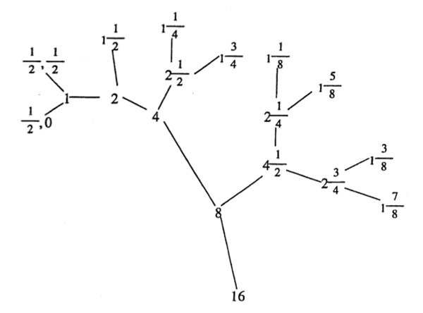
Now the intersection of these two groups is the modular subgroup $\Gamma_0(N) $ (consisting of those modular group element whose lower left-hand entry is divisible by N). That is, the proper way to look at this arithmetic group is as the joint stabilizer of the two lattices $L_1,L_N $. The picture makes it trivial to compute the index of this subgroup.

Consider the ball $B(L_1,N) $ with center $L_1 $ and hyper-radius N (on the left, the ball with hyper-radius 4). Then, it is easy to show that the modular group acts transitively on the boundary lattices (including the lattice $L_N $), whence the index $[ \Gamma : \Gamma_0(N)] $ is just the number of these boundary lattices. For N=4 the picture shows that there are exactly 6 of them. In general, it follows from our knowledge of all the p-trees the number of all lattices at hyperdistance N from $L_1 $ is equal to $N \prod_{p | N}(1+ \frac{1}{p}) $, in accordance with the well-known index formula for these modular subgroups!

But, there are many other applications of the big picture giving a simple interpretation for the Hecke operators, an elegant proof of the Atkin-Lehner theorem on the normalizer of $\Gamma_0(N) $ (the whimsical source of appearances of the number 24) and of Helling’s theorem characterizing maximal arithmetical groups inside $PSL_2(\mathbb{C}) $ as conjugates of the normalizers of $\Gamma_0(N) $ for square-free N.
J.H. Conway’s paper “Understanding groups like $\Gamma_0(N) $” containing all this material is a must-read! Unfortunately, I do not know of an online version.