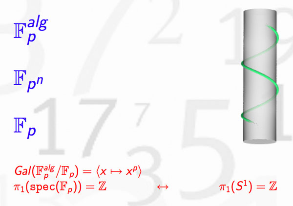
One of the more surprising analogies around is that prime numbers can be viewed as knots in the 3-sphere $S^3$. The motivation behind it is that the (etale) fundamental group of $\pmb{spec}(\mathbb{Z}/(p))$ is equal to (the completion) of the fundamental group of a circle $S^1$ and that the embedding
$\pmb{spec}(\mathbb{Z}/(p)) \subset \pmb{spec}(\mathbb{Z})$
embeds this circle as a knot in a 3-dimensional simply connected manifold which, after Perelman, has to be $S^3$. For more see the what is the knot associated to a prime?-post.
In recent months new evidence has come to light allowing us to settle the genesis of this marvelous idea.
1. The former consensus
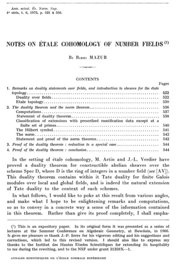
 Until now, the generally accepted view (see for example the ‘Mazur-dictionary-post’ or Morishita’s expository paper) was that the analogy between knots and primes was first pointed out by Barry Mazur in the middle of the 1960’s when preparing for his lectures at the Summer Conference on Algebraic Geometry, at Bowdoin, in 1966. The lecture notes where later published in 1973 in the Annales of the ENS as ‘Notes on etale cohomology of number fields’.
For further use in this series of posts, please note the acknowledgement at the bottom of the first page, reproduced below : “It gives me pleasure to thank J.-P. Serre for his vigorous editing and his suggestions and corrections, which led to this revised version.”
Independently, Yuri I. Manin spotted the same analogy at around the same time. However, this point of view was quickly forgotten in favor of the more classical one of viewing number fields as analogous to algebraic function fields of one variable. Subsequently, in the mid 1990’s Mikhail Kapranov and Alexander Reznikov took up the analogy between number fields and 3-manifolds again, and called the resulting study arithmetic topology.
2. The new evidence
On december 13th 2010, David Feldman posted a MathOverflow-question Mazur’s unpublished manuscript on primes and knots?. He wrote : “The story of the analogy between knots and primes, which now has a literature, started with an unpublished note by Barry Mazur. I’m not absolutely sure this is the one I mean, but in his paper, Analogies between group actions on 3-manifolds and number fields, Adam Sikora cites B. Mazur, Remarks on the Alexander polynomial, unpublished notes.“
Two months later, on february 15th David Feldman suddenly found the missing preprint in his mail-box and made it available. The preprint is now also available from Barry Mazur’s website. Mazur adds the following comment :
“In 1963 or 1964 I wrote an article Remarks on the Alexander Polynomial [PDF] about the analogy between knots in the three-dimensional sphere and prime numbers (and, correspondingly, the relationship between the Alexander polynomial and Iwasawa Theory). I distributed some copies of my article but never published it, and I misplaced my own copy. In subsequent years I have had many requests for my article and would often try to search through my files to find it, but never did. A few weeks ago Minh-Tri Do asked me for my article, and when I said I had none, he very kindly went on the web and magically found a scanned copy of it. I’m extremely grateful to Minh-Tri Do for his efforts (and many thanks, too, to David Feldman who provided the lead).”

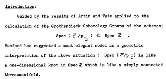
The opening paragraph of this unpublished preprint contains a major surprise!
Mazur points to David Mumford as the originator of the ‘primes-are-knots’ idea : “Mumford has suggested a most elegant model as a geometric interpretation of the above situation : $\pmb{spec}(\mathbb{Z}/p\mathbb{Z})$ is like a one-dimensional knot in $\pmb{spec}(\mathbb{Z})$ which is like a simply connected three-manifold.”
In a later post we will show that one can even pinpoint the time and place when and where this analogy was first dreamed-up to within a few days and a couple of miles.
For the impatient among you, have a sneak preview of the cradle of birth of the primes=knots idea…