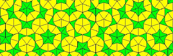
Skip to content →

Tag: geometry

Manin’s geometric axis

Mumford’s drawing has a clear emphasis on the vertical direction. The set of all vertical lines corresponds to taking the fibers of the natural ‘structural morphism’ : $\pi~:~\mathbf{spec}(\mathbb{Z}[t]) \rightarrow \mathbf{spec}(\mathbb{Z}) $ coming from the inclusion $\mathbb{Z} \subset \mathbb{Z}[t] $. That is, we consider the intersection $P \cap \mathbb{Z} $ of a prime ideal $P \subset \mathbb{Z}[t] $ with the subring of constants.

Two options arise : either $P \cap \mathbb{Z} \not= 0 $, in which case the intersection is a principal prime ideal $~(p) $ for some prime number $p $ (and hence $P $ itself is bigger or equal to $p\mathbb{Z}[t] $ whence its geometric object is contained in the vertical line $\mathbb{V}((p)) $, the fiber $\pi^{-1}((p)) $ of the structural morphism over $~(p) $), or, the intersection $P \cap \mathbb{Z}[t] = 0 $ reduces to the zero ideal (in which case the extended prime ideal $P \mathbb{Q}[x] = (q(x)) $ is a principal ideal of the rational polynomial algebra $\mathbb{Q}[x] $, and hence the geometric object corresponding to $P $ is a horizontal curve in Mumford’s drawing, or is the whole arithmetic plane itself if $P=0 $).

Because we know already that any ‘point’ in Mumford’s drawing corresponds to a maximal ideal of the form $\mathfrak{m}=(p,f(x)) $ (see last time), we see that every point lies on precisely one of the set of all vertical coordinate axes corresponding to the prime numbers ${~\mathbb{V}((p)) = \mathbf{spec}(\mathbb{F}_p[x]) = \pi^{-1}((p))~} $. In particular, two different vertical lines do not intersect (or, in ringtheoretic lingo, the ‘vertical’ prime ideals $p\mathbb{Z}[x] $ and $q\mathbb{Z}[x] $ are comaximal for different prime numbers $p \not= q $).


That is, the structural morphism is a projection onto the “arithmetic axis” (which is $\mathbf{spec}(\mathbb{Z}) $) and we get the above picture. The extra vertical line to the right of the picture is there because in arithmetic geometry it is customary to include also the archimedean valuations and hence to consider the ‘compactification’ of the arithmetic axis $\mathbf{spec}(\mathbb{Z}) $ which is $\overline{\mathbf{spec}(\mathbb{Z})} = \mathbf{spec}(\mathbb{Z}) \cup { v_{\mathbb{R}} } $.

Yuri I. Manin is advocating for years the point that we should take the terminology ‘arithmetic surface’ for $\mathbf{spec}(\mathbb{Z}[x]) $ a lot more seriously. That is, there ought to be, apart from the projection onto the ‘z-axis’ (that is, the arithmetic axis $\mathbf{spec}(\mathbb{Z}) $) also a projection onto the ‘x-axis’ which he calls the ‘geometric axis’.

But then, what are the ‘points’ of this geometric axis and what are their fibers under this second projection?

We have seen above that the vertical coordinate line over the prime number $~(p) $ coincides with $\mathbf{spec}(\mathbb{F}_p[x]) $, the affine line over the finite field $\mathbb{F}_p $. But all of these different lines, for varying primes $p $, should project down onto the same geometric axis. Manin’s idea was to take therefore as the geometric axis the affine line $\mathbf{spec}(\mathbb{F}_1[x]) $, over the virtual field with one element, which should be thought of as being the limit of the finite fields $\mathbb{F}_p $ when $p $ goes to one!

How many points does $\mathbf{spec}(\mathbb{F}_1[x]) $ have? Over a virtual object one can postulate whatever one wants and hope for an a posteriori explanation. $\mathbb{F}_1 $-gurus tell us that there should be exactly one point of size n on the affine line over $\mathbb{F}_1 $, corresponding to the unique degree n field extension $\mathbb{F}_{1^n} $. However, it is difficult to explain this from the limiting perspective…

Over a genuine finite field $\mathbb{F}_p $, the number of points of thickness $n $ (that is, those for which the residue field is isomorphic to the degree n extension $\mathbb{F}_{p^n} $) is equal to the number of monic irreducible polynomials of degree n over $\mathbb{F}_p $. This number is known to be $\frac{1}{n} \sum_{d | n} \mu(\frac{n}{d}) p^d $ where $\mu(k) $ is the Moebius function. But then, the limiting number should be $\frac{1}{n} \sum_{d | n} \mu(\frac{n}{d}) = \delta_{n1} $, that is, there can only be one point of size one…

Alternatively, one might consider the zeta function counting the number $N_n $ of ideals having a quotient consisting of precisely $p^n $ elements. Then, we have for genuine finite fields $\mathbb{F}_p $ that $\zeta(\mathbb{F}_p[x]) = \sum_{n=0}^{\infty} N_n t^n = 1 + p t + p^2 t^2 + p^3 t^3 + \ldots $, whence in the limit it should become
$1+t+t^2 +t^3 + \ldots $ and there is exactly one ideal in $\mathbb{F}_1[x] $ having a quotient of cardinality n and one argues that this unique quotient should be the unique point with residue field $\mathbb{F}_{1^n} $ (though it might make more sense to view this as the unique n-fold extension of the unique size-one point $\mathbb{F}_1 $ corresponding to the quotient $\mathbb{F}_1[x]/(x^n) $…)

A perhaps more convincing reasoning goes as follows. If $\overline{\mathbb{F}_p} $ is an algebraic closure of the finite field $\mathbb{F}_p $, then the points of the affine line over $\overline{\mathbb{F}_p} $ are in one-to-one correspondence with the maximal ideals of $\overline{\mathbb{F}_p}[x] $ which are all of the form $~(x-\lambda) $ for $\lambda \in \overline{\mathbb{F}_p} $. Hence, we get the points of the affine line over the basefield $\mathbb{F}_p $ as the orbits of points over the algebraic closure under the action of the Galois group $Gal(\overline{\mathbb{F}_p}/\mathbb{F}_p) $.

‘Common wisdom’ has it that one should identify the algebraic closure of the field with one element $\overline{\mathbb{F}_{1}} $ with the group of all roots of unity $\mathbb{\mu}_{\infty} $ and the corresponding Galois group $Gal(\overline{\mathbb{F}_{1}}/\mathbb{F}_1) $ as being generated by the power-maps $\lambda \rightarrow \lambda^n $ on the roots of unity. But then there is exactly one orbit of length n given by the n-th roots of unity $\mathbb{\mu}_n $, so there should be exactly one point of thickness n in $\mathbf{spec}(\mathbb{F}_1[x]) $ and we should then identity the corresponding residue field as $\mathbb{F}_{1^n} = \mathbb{\mu}_n $.

Whatever convinces you, let us assume that we can identify the non-generic points of $\mathbf{spec}(\mathbb{F}_1[x]) $ with the set of positive natural numbers ${ 1,2,3,\ldots } $ with $n $ denoting the unique size n point with residue field $\mathbb{F}_{1^n} $. Then, what are the fibers of the projection onto the geometric axis $\phi~:~\mathbf{spec}(\mathbb{Z}[x]) \rightarrow \mathbf{spec}(\mathbb{F}_1[x]) = { 1,2,3,\ldots } $?

These fibers should correspond to ‘horizontal’ principal prime ideals of $\mathbb{Z}[x] $. Manin proposes to consider $\phi^{-1}(n) = \mathbb{V}((\Phi_n(x))) $ where $\Phi_n(x) $ is the n-th cyclotomic polynomial. The nice thing about this proposal is that all closed points of $\mathbf{spec}(\mathbb{Z}[x]) $ lie on one of these fibers!

Indeed, the residue field at such a point (corresponding to a maximal ideal $\mathfrak{m}=(p,f(x)) $) is the finite field $\mathbb{F}_{p^n} $ and as all its elements are either zero or an $p^n-1 $-th root of unity, it does lie on the curve determined by $\Phi_{p^n-1}(x) $.

As a consequence, the localization $\mathbb{Z}[x]_{cycl} $ of the integral polynomial ring $\mathbb{Z}[x] $ at the multiplicative system generated by all cyclotomic polynomials is a principal ideal domain (as all height two primes evaporate in the localization), and, the fiber over the generic point of $\mathbf{spec}(\mathbb{F}_1[x]) $ is $\mathbf{spec}(\mathbb{Z}[x]_{cycl}) $, which should be compared to the fact that the fiber of the generic point in the projection onto the arithmetic axis is $\mathbf{spec}(\mathbb{Q}[x]) $ and $\mathbb{Q}[x] $ is the localization of $\mathbb{Z}[x] $ at the multiplicative system generated by all prime numbers).

Hence, both the vertical coordinate lines and the horizontal ‘lines’ contain all closed points of the arithmetic plane. Further, any such closed point $\mathfrak{m}=(p,f(x)) $ lies on the intersection of a vertical line $\mathbb{V}((p)) $ and a horizontal one $\mathbb{V}((\Phi_{p^n-1}(x))) $ (if $deg(f(x))=n $).
That is, these horizontal and vertical lines form a coordinate system, at least for the closed points of $\mathbf{spec}(\mathbb{Z}[x]) $.

Still, there is a noticeable difference between the two sets of coordinate lines. The vertical lines do not intersect meaning that $p\mathbb{Z}[x]+q\mathbb{Z}[x]=\mathbb{Z}[x] $ for different prime numbers p and q. However, in general the principal prime ideals corresponding to the horizontal lines $~(\Phi_n(x)) $ and $~(\Phi_m(x)) $ are not comaximal when $n \not= m $, that is, these ‘lines’ may have points in common! This will lead to an exotic new topology on the roots of unity… (to be continued).

Leave a Comment

Mumford’s treasure map


David Mumford did receive earlier this year the 2007 AMS Leroy P. Steele Prize for Mathematical Exposition. The jury honors Mumford for “his beautiful expository accounts of a host of aspects of algebraic geometry”. Not surprisingly, the first work they mention are his mimeographed notes of the first 3 chapters of a course in algebraic geometry, usually called “Mumford’s red book” because the notes were wrapped in a red cover. In 1988, the notes were reprinted by Springer-Verlag. Unfortnately, the only red they preserved was in the title.

The AMS describes the importance of the red book as follows. “This is one of the few books that attempt to convey in pictures some of the highly abstract notions that arise in the field of algebraic geometry. In his response upon receiving the prize, Mumford recalled that some of his drawings from The Red Book were included in a collection called Five Centuries of French Mathematics. This seemed fitting, he noted: “After all, it was the French who started impressionist painting and isn’t this just an impressionist scheme for rendering geometry?””

These days it is perfectly possible to get a good grasp on difficult concepts from algebraic geometry by reading blogs, watching YouTube or plugging in equations to sophisticated math-programs. In the early seventies though, if you wanted to know what Grothendieck’s scheme-revolution was all about you had no choice but to wade through the EGA’s and SGA’s and they were notorious for being extremely user-unfriendly regarding illustrations…

So the few depictions of schemes available, drawn by people sufficiently fluent in Grothendieck’s new geometric language had no less than treasure-map-cult-status and were studied in minute detail. Mumford’s red book was a gold mine for such treasure maps. Here’s my favorite one, scanned from the original mimeographed notes (it looks somewhat tidier in the Springer-version)


It is the first depiction of $\mathbf{spec}(\mathbb{Z}[x]) $, the affine scheme of the ring $\mathbb{Z}[x] $ of all integral polynomials. Mumford calls it the”arithmetic surface” as the picture resembles the one he made before of the affine scheme $\mathbf{spec}(\mathbb{C}[x,y]) $ corresponding to the two-dimensional complex affine space $\mathbb{A}^2_{\mathbb{C}} $. Mumford adds that the arithmetic surface is ‘the first example which has a real mixing of arithmetic and geometric properties’.

Let’s have a closer look at the treasure map. It introduces some new signs which must have looked exotic at the time, but have since become standard tools to depict algebraic schemes.

For starters, recall that the underlying topological space of $\mathbf{spec}(\mathbb{Z}[x]) $ is the set of all prime ideals of the integral polynomial ring $\mathbb{Z}[x] $, so the map tries to list them all as well as their inclusions/intersections.

The doodle in the right upper corner depicts the ‘generic point’ of the scheme. That is, the geometric object corresponding to the prime ideal $~(0) $ (note that $\mathbb{Z}[x] $ is an integral domain). Because the zero ideal is contained in any other prime ideal, the algebraic/geometric mantra (“inclusions reverse when shifting between algebra and geometry”) asserts that the gemetric object corresponding to $~(0) $ should contain all other geometric objects of the arithmetic plane, so it is just the whole plane! Clearly, it is rather senseless to depict this fact by coloring the whole plane black as then we wouldn’t be able to see the finer objects. Mumford’s solution to this is to draw a hairy ball, which in this case, is sufficiently thick to include fragments going in every possible direction. In general, one should read these doodles as saying that the geometric object represented by this doodle contains all other objects seen elsewhere in the picture if the hairy-ball-doodle includes stuff pointing in the direction of the smaller object. So, in the case of the object corresponding to $~(0) $, the doodle has pointers going everywhere, saying that the geometric object contains all other objects depicted.

Let’s move over to the doodles in the lower right-hand corner. They represent the geometric object corresponding to principal prime ideals of the form $~(p(x)) $, where $p(x) $ in an irreducible polynomial over the integers, that is, a polynomial which we cannot write as the product of two smaller integral polynomials. The objects corresponding to such prime ideals should be thought of as ‘horizontal’ curves in the plane.

The doodles depicted correspond to the prime ideal $~(x) $, containing all polynomials divisible by $x $ so when we divide it out we get, as expected, a domain $\mathbb{Z}[x]/(x) \simeq \mathbb{Z} $, and the one corresponding to the ideal $~(x^2+1) $, containing all polynomials divisible by $x^2+1 $, which can be proved to be a prime ideals of $\mathbb{Z}[x] $ by observing that after factoring out we get $\mathbb{Z}[x]/(x^2+1) \simeq \mathbb{Z}[i] $, the domain of all Gaussian integers $\mathbb{Z}[i] $. The corresponding doodles (the ‘generic points’ of the curvy-objects) have a predominant horizontal component as they have the express the fact that they depict horizontal curves in the plane. It is no coincidence that the doodle of $~(x^2+1) $ is somewhat bulkier than the one of $~(x) $ as the later one must only depict the fact that all points lying on the straight line to its left belong to it, whereas the former one must claim inclusion of all points lying on the ‘quadric’ it determines.

Apart from these ‘horizontal’ curves, there are also ‘vertical’ lines corresponding to the principal prime ideals $~(p) $, containing the polynomials, all of which coefficients are divisible by the prime number $p $. These are indeed prime ideals of $\mathbb{Z}[x] $, because their quotients are
$\mathbb{Z}[x]/(p) \simeq (\mathbb{Z}/p\mathbb{Z})[x] $ are domains, being the ring of polynomials over the finite field $\mathbb{Z}/p\mathbb{Z} = \mathbb{F}_p $. The doodles corresponding to these prime ideals have a predominant vertical component (depicting the ‘vertical’ lines) and have a uniform thickness for all prime numbers $p $ as each of them only has to claim ownership of the points lying on the vertical line under them.

Right! So far we managed to depict the zero prime ideal (the whole plane) and the principal prime ideals of $\mathbb{Z}[x] $ (the horizontal curves and the vertical lines). Remains to depict the maximal ideals. These are all known to be of the form
$\mathfrak{m} = (p,f(x)) $
where $p $ is a prime number and $f(x) $ is an irreducible integral polynomial, which remains irreducible when reduced modulo $p $ (that is, if we reduce all coefficients of the integral polynomial $f(x) $ modulo $p $ we obtain an irreducible polynomial in $~\mathbb{F}_p[x] $). By the algebra/geometry mantra mentioned before, the geometric object corresponding to such a maximal ideal can be seen as the ‘intersection’ of an horizontal curve (the object corresponding to the principal prime ideal $~(f(x)) $) and a vertical line (corresponding to the prime ideal $~(p) $). Because maximal ideals do not contain any other prime ideals, there is no reason to have a doodle associated to $\mathfrak{m} $ and we can just depict it by a “point” in the plane, more precisely the intersection-point of the horizontal curve with the vertical line determined by $\mathfrak{m}=(p,f(x)) $. Still, Mumford’s treasure map doesn’t treat all “points” equally. For example, the point corresponding to the maximal ideal $\mathfrak{m}_1 = (3,x+2) $ is depicted by a solid dot $\mathbf{.} $, whereas the point corresponding to the maximal ideal $\mathfrak{m}_2 = (3,x^2+1) $ is represented by a fatter point $\circ $. The distinction between the two ‘points’ becomes evident when we look at the corresponding quotients (which we know have to be fields). We have

$\mathbb{Z}[x]/\mathfrak{m}_1 = \mathbb{Z}[x]/(3,x+2)=(\mathbb{Z}/3\mathbb{Z})[x]/(x+2) = \mathbb{Z}/3\mathbb{Z} = \mathbb{F}_3 $ whereas $\mathbb{Z}[x]/\mathfrak{m}_2 = \mathbb{Z}[x]/(3,x^2+1) = \mathbb{Z}/3\mathbb{Z}[x]/(x^2+1) = \mathbb{F}_3[x]/(x^2+1) = \mathbb{F}_{3^2} $

because the polynomial $x^2+1 $ remains irreducible over $\mathbb{F}_3 $, the quotient $\mathbb{F}_3[x]/(x^2+1) $ is no longer the prime-field $\mathbb{F}_3 $ but a quadratic field extension of it, that is, the finite field consisting of 9 elements $\mathbb{F}_{3^2} $. That is, we represent the ‘points’ lying on the vertical line corresponding to the principal prime ideal $~(p) $ by a solid dot . when their quotient (aka residue field is the prime field $~\mathbb{F}_p $, by a bigger point $\circ $ when its residue field is the finite field $~\mathbb{F}_{p^2} $, by an even fatter point $\bigcirc $ when its residue field is $~\mathbb{F}_{p^3} $ and so on, and on. The larger the residue field, the ‘fatter’ the corresponding point.

In fact, the ‘fat-point’ signs in Mumford’s treasure map are an attempt to depict the fact that an affine scheme contains a lot more information than just the set of all prime ideals. In fact, an affine scheme determines (and is determined by) a “functor of points”. That is, to every field (or even every commutative ring) the affine scheme assigns the set of its ‘points’ defined over that field (or ring). For example, the $~\mathbb{F}_p $-points of $\mathbf{spec}(\mathbb{Z}[x]) $ are the solid . points on the vertical line $~(p) $, the $~\mathbb{F}_{p^2} $-points of $\mathbf{spec}(\mathbb{Z}[x]) $ are the solid . points and the slightly bigger $\circ $ points on that vertical line, and so on.

This concludes our first attempt to decypher Mumford’s drawing, but if we delve a bit deeper, we are bound to find even more treasures… (to be continued).

5 Comments

noncommutative F_un geometry (2)

Last time we tried to generalize the Connes-Consani approach to commutative algebraic geometry over the field with one element $\mathbb{F}_1 $ to the noncommutative world by considering covariant functors

$N~:~\mathbf{groups} \rightarrow \mathbf{sets} $

which over $\mathbb{C} $ resp. $\mathbb{Z} $ become visible by a complex (resp. integral) algebra having suitable universal properties.

However, we didn’t specify what we meant by a complex noncommutative variety (resp. an integral noncommutative scheme). In particular, we claimed that the $\mathbb{F}_1 $-‘points’ associated to the functor

$D~:~\mathbf{groups} \rightarrow \mathbf{sets} \qquad G \mapsto G_2 \times G_3 $ (here $G_n $ denotes all elements of order $n $ of $G $)

were precisely the modular dessins d’enfants of Grothendieck, but didn’t give details. We’ll try to do this now.

For algebras over a field we follow the definition, due to Kontsevich and Soibelman, of so called “noncommutative thin schemes”. Actually, the thinness-condition is implicit in both Soule’s-approach as that of Connes and Consani : we do not consider R-points in general, but only those of rings R which are finite and flat over our basering (or field).

So, what is a noncommutative thin scheme anyway? Well, its a covariant functor (commuting with finite projective limits)

$\mathbb{X}~:~\mathbf{Alg}^{fd}_k \rightarrow \mathbf{sets} $

from finite-dimensional (possibly noncommutative) $k $-algebras to sets. Now, the usual dual-space operator gives an anti-equivalence of categories

$\mathbf{Alg}^{fd}_k \leftrightarrow \mathbf{Coalg}^{fd}_k \qquad A=C^* \leftrightarrow C=A^* $

so a thin scheme can also be viewed as a contra-variant functor (commuting with finite direct limits)

$\mathbb{X}~:~\mathbf{Coalg}^{fd}_k \rightarrow \mathbf{Sets} $

In particular, we are interested to associated to any {tex]k $-algebra $A $ its representation functor :

$\mathbf{rep}(A)~:~\mathbf{Coalg}^{fd}_k \rightarrow \mathbf{Sets} \qquad C \mapsto Alg_k(A,C^*) $

This may look strange at first sight, but $C^* $ is a finite dimensional algebra and any $n $-dimensional representation of $A $ is an algebra map $A \rightarrow M_n(k) $ and we take $C $ to be the dual coalgebra of this image.

Kontsevich and Soibelman proved that every noncommutative thin scheme $\mathbb{X} $ is representable by a $k $-coalgebra. That is, there exists a unique coalgebra $C_{\mathbb{X}} $ (which they call the coalgebra of ‘distributions’ of $\mathbb{X} $) such that for every finite dimensional $k $-algebra $B $ we have

$\mathbb{X}(B) = Coalg_k(B^*,C_{\mathbb{X}}) $

In the case of interest to us, that is for the functor $\mathbf{rep}(A) $ the coalgebra of distributions is Kostant’s dual coalgebra $A^o $. This is the not the full linear dual of $A $ but contains only those linear functionals on $A $ which factor through a finite dimensional quotient.

So? You’ve exchanged an algebra $A $ for some coalgebra $A^o $, but where’s the geometry in all this? Well, let’s look at the commutative case. Suppose $A= \mathbb{C}[X] $ is the coordinate ring of a smooth affine variety $X $, then its dual coalgebra looks like

$\mathbb{C}[X]^o = \oplus_{x \in X} U(T_x(X)) $

the direct sum of all universal (co)algebras of tangent spaces at points $x \in X $. But how do we get the variety out of this? Well, any coalgebra has a coradical (being the sun of all simple subcoalgebras) and in the case just mentioned we have

$corad(\mathbb{C}[X]^o) = \oplus_{x \in X} \mathbb{C} e_x $

so every point corresponds to a unique simple component of the coradical. In the general case, the coradical of the dual coalgebra $A^o $ is the direct sum of all simple finite dimensional representations of $A $. That is, the direct summands of the coalgebra give us a noncommutative variety whose points are the simple representations, and the remainder of the coalgebra of distributions accounts for infinitesimal information on these points (as do the tangent spaces in the commutative case).

In fact, it was a surprise to me that one can describe the dual coalgebra quite explicitly, and that $A_{\infty} $-structures make their appearance quite naturally. See this paper if you’re in for the details on this.

That settles the problem of what we mean by the noncommutative variety associated to a complex algebra. But what about the integral case? In the above, we used extensively the theory of Kostant-duality which works only for algebras over fields…

Well, not quite. In the case of $\mathbb{Z} $ (or more general, of Dedekind domains) one can repeat Kostant’s proof word for word provided one takes as the definition of the dual $\mathbb{Z} $-coalgebra
of an algebra (which is $\mathbb{Z} $-torsion free)

$A^o = { f~:~A \rightarrow \mathbb{Z}~:~A/Ker(f)~\text{is finitely generated and torsion free}~} $

(over general rings there may be also variants of this duality, as in Street’s book an Quantum groups). Probably lots of people have come up with this, but the only explicit reference I have is to the first paper I’ve ever written. So, also for algebras over $\mathbb{Z} $ we can define a suitable noncommutative integral scheme (the coradical approach accounts only for the maximal ideals rather than all primes, but somehow this is implicit in all approaches as we consider only thin schemes).

Fine! So, we can make sense of the noncommutative geometrical objects corresponding to the group-algebras $\mathbb{C} \Gamma $ and $\mathbb{Z} \Gamma $ where $\Gamma = PSL_2(\mathbb{Z}) $ is the modular group (the algebras corresponding to the $G \mapsto G_2 \times G_3 $-functor). But, what might be the points of the noncommutative scheme corresponding to $\mathbb{F}_1 \Gamma $???

Well, let’s continue the path cut out before. “Points” should correspond to finite dimensional “simple representations”. Hence, what are the finite dimensional simple $\mathbb{F}_1 $-representations of $\Gamma $? (Or, for that matter, of any group $G $)

Here we come back to Javier’s post on this : a finite dimensional $\mathbb{F}_1 $-vectorspace is a finite set. A $\Gamma $-representation on this set (of n-elements) is a group-morphism

$\Gamma \rightarrow GL_n(\mathbb{F}_1) = S_n $

hence it gives a permutation representation of $\Gamma $ on this set. But then, if finite dimensional $\mathbb{F}_1 $-representations of $\Gamma $ are the finite permutation representations, then the simple ones are the transitive permutation representations. That is, the points of the noncommutative scheme corresponding to $\mathbb{F}_1 \Gamma $ are the conjugacy classes of subgroups $H \subset \Gamma $ such that $\Gamma/H $ is finite. But these are exactly the modular dessins d’enfants introduced by Grothendieck as I explained a while back elsewhere (see for example this post and others in the same series).

Leave a Comment

noncommutative F_un geometry (1)

It is perhaps surprising that Alain Connes and Katia Consani, two icons of noncommutative geometry, restrict themselves to define commutative algebraic geometry over $\mathbb{F}_1 $, the field with one element.

My guess of why they stop there is as good as anyone’s. Perhaps they felt that there is already enough noncommutativity in Soule’s gadget-approach (the algebra $\mathcal{A}_X $ as in this post may very well be noncommutative). Perhaps they were only interested in the Bost-Connes system which can be entirely encoded in their commutative $\mathbb{F}_1 $-geometry. Perhaps they felt unsure as to what the noncommutative scheme of an affine noncommutative algebra might be. Perhaps …

Remains the fact that their approach screams for a noncommutative extension. Their basic object is a covariant functor

$N~:~\mathbf{abelian} \rightarrow \mathbf{sets} \qquad A \mapsto N(A) $

from finite abelian groups to sets, together with additional data to the effect that there is a unique minimal integral scheme associated to $N $. In a series of posts on the Connes-Consani paper (starting here) I took some care of getting rid of all scheme-lingo and rephrasing everything entirely into algebras. But then, this set-up can be extended verbatim to noncommuative $\mathbb{F}_1 $-geometry, which should start from a covariant functor

$N~:~\mathbf{groups} \rightarrow \mathbf{sets} $

from all finite groups to sets. Let’s recall quickly what the additional info should be making this functor a noncommutative (affine) F_un scheme :

There should be a finitely generated $\mathbb{C} $-algebra $R $ together with a natural transformation (the ‘evaluation’)

$e~:~N \rightarrow \mathbf{maxi}(R) \qquad N(G) \mapsto Hom_{\mathbb{C}-alg}(R, \mathbb{C} G) $

(both $R $ and the group-algebra $\mathbb{C} G $ may be noncommutative). The pair $(N, \mathbf{maxi}(R)) $ is then called a gadget and there is an obvious notion of ‘morphism’ between gadgets.

The crucial extra ingredient is an affine $\mathbb{Z} $-algebra (possibly noncommutative) $S $
such that $N $ is a subfunctor of $\mathbf{mini}(S)~:~G \mapsto Hom_{\mathbb{Z}-alg}(S,\mathbb{Z} G) $ together with the following universal property :

any affine $\mathbb{Z} $-algebra $T $ having a gadget-morphism $~(N,\mathbf{maxi}(R)) \rightarrow (\mathbf{mini}(T),\mathbf{maxi}(T \otimes_{\mathbb{Z}} \mathbb{C})) $ comes from a $\mathbb{Z} $-algebra morphism $T \rightarrow S $. (If this sounds too cryptic for you, please read the series on C-C mentioned before).

So, there is no problem in defining noncommutative affine F_un-schemes. However, as with any generalization, this only makes sense provided (a) we get something new and (b) we have interesting examples, not covered by the restricted theory.

At first sight we do not get something new as in the only example we did in the C-C-series (the forgetful functor) it is easy to prove (using the same proof as given in this post) that the forgetful-functor $\mathbf{groups} \rightarrow \mathbf{sets} $ still has as its integral form the integral torus $\mathbb{Z}[x,x^{-1}] $. However, both theories quickly diverge beyond this example.

For example, consider the functor

$\mathbf{groups} \rightarrow \mathbf{sets} \qquad G \mapsto G \times G $

Then, if we restrict to abelian finite groups $\mathbf{abelian} $ it is easy to see (again by a similar argument) that the two-dimensional integer torus $\mathbb{Z}[x,y,x^{-1},y^{-1}] $ is the correct integral form. However, this algebra cannot be the correct form for the functor on the category of all finite groups as any $\mathbb{Z} $-algebra map $\phi~:~\mathbb{Z}[x,y,x^{-1},y^{-1}] \rightarrow \mathbb{Z} G $ determines (and is determined by) a pair of commuting units in $\mathbb{Z} G $, so the above functor can not be a subfunctor if we allow non-Abelian groups.

But then, perhaps there isn’t a minimal integral $\mathbb{Z} $-form for this functor? Well, yes there is. Take the free group in two letters (that is, all words in noncommuting $x,y,x^{-1} $ and $y^{-1} $ satisfying only the trivial cancellation laws between a letter and its inverse), then the corresponding integral group-algebra $\mathbb{Z} \mathcal{F}_2 $ does the trick.

Again, the proof-strategy is the same. Given a gadget-morphism we have an algebra map $f~:~T \mapsto \mathbb{C} \mathcal{F}_2 $ and we have to show, using the universal property that the image of $T $ is contained in the integral group-algebra $\mathbb{Z} \mathcal{F}_2 $. Take a generator
$z $ of $T $ then the degree of the image $f(z) $ is bounded say by $d $ and we can always find a subgroup $H \subset \mathcal{F}_2 $ such that $\mathcal{F}_2/H $ is a fnite group and the quotient map $\mathbb{C} \mathcal{F}_2 \rightarrow \mathbb{C} \mathcal{F}_2/H $ is injective on the subspace spanned by all words of degree strictly less than $d+1 $. Then, the usual diagram-chase finishes the proof.

What makes this work is that the free group $\mathcal{F}_2 $ has ‘enough’ subgroups of finite index, a property it shares with many interesting discrete groups. Whence the blurb-message :

if the integers $\mathbb{Z} $ see a discrete group $\Gamma $, then the field $\mathbb{F}_1 $ sees its profinite completion $\hat{\Gamma} = \underset{\leftarrow}{lim}~\Gamma/ H $

So, yes, we get something new by extending the Connes-Consani approach to the noncommutative world, but do we have interesting examples? As “interesting” is a subjective qualification, we’d better invoke the authority-argument.

Alexander Grothendieck (sitting on the right, manifestly not disputing a vacant chair with Jean-Pierre Serre, drinking on the left (a marvelous picture taken by F. Hirzebruch in 1958)) was pushing the idea that profinite completions of arithmetical groups were useful in the study of the absolute Galois group $Gal(\overline{\mathbb{Q}}/\mathbb{Q}) $, via his theory of dessins d’enfants (children;s drawings).

In a previous life, I’ve written a series of posts on dessins d’enfants, so I’ll restrict here to the basics. A smooth projective $\overline{\mathbb{Q}} $-curve $X $ has a Belyi-map $X \rightarrow \mathbb{P}^1_{\overline{\mathbb{Q}}} $ ramified only in three points ${ 0,1,\infty } $. The “drawing” corresponding to $X $ is a bipartite graph, drawn on the Riemann surface $X_{\mathbb{C}} $ obtained by lifting the unit interval $[0,1] $ to $X $. As the absolute Galois group acts on all such curves (and hence on their corresponding drawings), the action of it on these dessins d’enfants may give us a way into the multiple mysteries of the absolute Galois group.

In his “Esquisse d’un programme” (Sketch of a program if you prefer to read it in English) he writes :

“C’est ainsi que mon attention s’est portée vers ce que j’ai appelé depuis la “géométrie algêbrique anabélienne”, dont le point de départ est justement une étude (pour le moment limitée à la caractéristique zéro) de l’action de groupe de Galois “absolus” (notamment les groupes $Gal(\overline{K}/K) $, ou $K $ est une extension de type fini du corps premier) sur des groupes fondamentaux géométriques (profinis) de variétés algébriques (définies sur $K $), et plus particulièrement (rompant avec une tradition bien enracinée) des groupes fondamentaux qui sont trés éloignés des groupes abéliens (et que pour cette raison je nomme “anabéliens”). Parmi ces groupes, et trés proche du groupe $\hat{\pi}_{0,3} $, il y a le compactifié profini du groupe modulaire $SL_2(\mathbb{Z}) $, dont le quotient par le centre $\pm 1 $ contient le précédent comme sous-groupe de congruence mod 2, et peut s’interpréter d’ailleurs comme groupe “cartographique” orienté, savoir celui qui classifie les cartes orientées triangulées (i.e. celles dont les faces des triangles ou des monogones).”

and a bit further, he writes :

“L’élément de structure de $SL_2(\mathbb{Z}) $ qui me fascine avant tout, est bien sur l’action extérieure du groupe de Galois $Gal(\overline{\mathbb{Q}}/\mathbb{Q}) $ sur le compactifié profini. Par le théorème de Bielyi, prenant les compactifiés profinis de sous-groupes d’indice fini de $SL_2(\mathbb{Z}) $, et l’action extérieure induite (quitte à passer également à un sous-groupe overt de $Gal(\overline{\mathbb{Q}},\mathbb{Q}) $), on trouve essentiellement les groupes fondamentaux de toutes les courbes algébriques définis sur des corps de nombres $K $, et l’action extérieure de $Gal(\overline{K}/K) $ dessus.”

So, is there a noncommutative affine variety over $\mathbb{F}_1 $ of which the unique minimal integral model is the integral group algebra of the modular group $\mathbb{Z} \Gamma $ (with $\Gamma = PSL_2(\mathbb{Z}) $? Yes, here it is

$N_{\Gamma}~:~\mathbf{groups} \rightarrow \mathbf{sets} \qquad G \mapsto G_2 \times G_3 $

where $G_n $ is the set of all elements of order $n $ in $G $. The reason behind this is that the modular group is the free group product $C_2 \ast C_3 $.

Fine, you may say, but all this is just algebra. Where is the noncommutative complex variety or the noncommutative integral scheme in all this? Well, we can introduce them too but as this post is already 1300 words long, I’ll better leave this for another time. In case you cannot stop thinking about it, here’s the short answer.

The complex noncommutative variety has as its ‘points’ all finite dimensional simple complex representations of the modular group, and the ‘points’ of the noncommutative $\mathbb{F}_1 $-scheme are exactly the (modular) dessins d’enfants…

Leave a Comment

This week at F_un Mathematics (1)

In case you haven’t noticed it yet : I’m not living here anymore.

My blogging is (at least for the moment) transfered to the F_un Mathematics blog which some prefer to call the “ceci n’est pas un corps”-blog, which is very fine with me.

Javier gave a talk at MPI on Soule’s approach to algebraic geometry over the elusive field with one element $\mathbb{F}_1 $ and wrote two posts about it The skeleton of Soule’s F_un geometry and Gadgets a la Soule. The rough idea being that a variety over the field with one element only acquires flesh after a base extension to $\mathbb{Z} $ and to cyclotomic integers.

I did some posts on a related (but conceptually somewhat easier) approach due to Alain Connes and Katia Consani. I’ve tried to explain their construction at the level of (mature) undergraduate students. So far, there are three posts part1, part2 and part3. Probably there is one more session to come in which I will explain why they need functors to graded sets.

In the weeks to come we plan to post about applications of this F_un-geometry to noncommutative geometry (the Bost-Connes system) and Grothendieck’s anabelian geometry (the theory of dessins d’enfant). I’ll try to leave a short account of the main posts here, but clearly you are invited to feed your feedreader this.

Perhaps I’ll return here for a week mid november to do some old-fashioned vacation blogging. I have to admit I did underestimate Numeo.fr. Rumours have it that our place is connected wirelessly to the web…

Leave a Comment

Connes-Consani for undergraduates (3)

A quick recap of last time. We are trying to make sense of affine varieties over the elusive field with one element $\mathbb{F}_1 $, which by Grothendieck’s scheme-philosophy should determine a functor

$\mathbf{nano}(N)~:~\mathbf{abelian} \rightarrow \mathbf{sets} \qquad A \mapsto N(A) $

from finite Abelian groups to sets, typically giving pretty small sets $N(A) $. Using the F_un mantra that $\mathbb{Z} $ should be an algebra over $\mathbb{F}_1 $ any $\mathbb{F}_1 $-variety determines an integral scheme by extension of scalars, as well as a complex variety (by extending further to $\mathbb{C} $). We have already connected the complex variety with the original functor into a gadget that is a couple $~(\mathbf{nano}(N),\mathbf{maxi}(R)) $ where $R $ is the coordinate ring of a complex affine variety $X_R $ having the property that every element of $N(A) $ can be realized as a $\mathbb{C} A $-point of $X_R $. Ringtheoretically this simply means that to every element $x \in N(A) $ there is an algebra map $N_x~:~R \rightarrow \mathbb{C} A $.

Today we will determine which gadgets determine an integral scheme, and do so uniquely, and call them the sought for affine schemes over $\mathbb{F}_1 $.

Let’s begin with our example : $\mathbf{nano}(N) = \underline{\mathbb{G}}_m $ being the forgetful functor, that is $N(A)=A $ for every finite Abelian group, then the complex algebra $R= \mathbb{C}[x,x^{-1}] $ partners up to form a gadget because to every element $a \in N(A)=A $ there is a natural algebra map $N_a~:~\mathbb{C}[x,x^{-1}] \rightarrow \mathbb{C} A $ defined by sending $x \mapsto e_a $. Clearly, there is an obvious integral form of this complex algebra, namely $\mathbb{Z}[x,x^{-1}] $ but we have already seen that this algebra represents the mini-functor

$\mathbf{min}(\mathbb{Z}[x,x^{-1}])~:~\mathbf{abelian} \rightarrow \mathbf{sets} \qquad A \mapsto (\mathbb{Z} A)^* $

and that the group of units $(\mathbb{Z} A)^* $ of the integral group ring $\mathbb{Z} A $ usually is a lot bigger than $N(A)=A $. So, perhaps there is another less obvious $\mathbb{Z} $-algebra $S $ doing a much better job at approximating $N $? That is, if we can formulate this more precisely…

In general, every $\mathbb{Z} $-algebra $S $ defines a gadget $\mathbf{gadget}(S) = (\mathbf{mini}(S),\mathbf{maxi}(S \otimes_{\mathbb{Z}} \mathbb{C})) $ with the obvious (that is, extension of scalars) evaluation map

$\mathbf{mini}(S)(A) = Hom_{\mathbb{Z}-alg}(S, \mathbb{Z} A) \rightarrow Hom_{\mathbb{C}-alg}(S \otimes_{\mathbb{Z}} \mathbb{C}, \mathbb{C} A) = \mathbf{maxi}(S \otimes_{\mathbb{Z}} \mathbb{C})(A) $

Right, so how might one express the fact that the integral affine scheme $X_T $ with integral algebra $T $ is the ‘best’ integral approximation of a gadget $~(\mathbf{nano}(N),\mathbf{maxi}(R)) $. Well, to begin its representing functor should at least contain the information given by $N $, that is, $\mathbf{nano}(N) $ is a sub-functor of $\mathbf{mini}(T) $ (meaning that for every finite Abelian group $A $ we have a natural inclusion $N(A) \subset Hom_{\mathbb{Z}-alg}(T, \mathbb{Z} A) $). As to the “best”-part, we must express that all other candidates factor through $T $. That is, suppose we have an integral algebra $S $ and a morphism of gadgets (as defined last time)

$f~:~(\mathbf{nano}(N),\mathbf{maxi}(R)) \rightarrow \mathbf{gadget}(S) = (\mathbf{mini}(S),\mathbf{maxi}(S \otimes_{\mathbb{Z}} \mathbb{C})) $

then there ought to be $\mathbb{Z} $-algebra morphism $T \rightarrow S $ such that the above map $f $ factors through an induced gadget-map $\mathbf{gadget}(T) \rightarrow \mathbf{gadget}(S) $.

Fine, but is this definition good enough in our trivial example? In other words, is the “obvious” integral ring $\mathbb{Z}[x,x^{-1}] $ the best integral choice for approximating the forgetful functor $N=\underline{\mathbb{G}}_m $? Well, take any finitely generated integral algebra $S $, then saying that there is a morphism of gadgets from $~(\underline{\mathbb{G}}_m,\mathbf{maxi}(\mathbb{C}[x,x^{-1}]) $ to $\mathbf{gadget}(S) $ means that there is a $\mathbb{C} $-algebra map $\psi~:~S \otimes_{\mathbb{Z}} \mathbb{C} \rightarrow \mathbb{C}[x,x^{-1}] $ such that for every finite Abelian group $A $ we have a commuting diagram

$\xymatrix{A \ar[rr] \ar[d]_e & & Hom_{\mathbb{Z}-alg}(S, \mathbb{Z} A) \ar[d] \\
Hom_{\mathbb{C}-alg}(\mathbb{C}[x,x^{-1}],\mathbb{C} A) \ar[rr]^{- \circ \psi} & & Hom_{\mathbb{C}-alg}(S \otimes_{\mathbb{Z}} \mathbb{C}, \mathbb{C} A)} $

Here, $e $ is the natural evaluation map defined before sending a group-element $a \in A $ to the algebra map defined by $x \mapsto e_a $ and the vertical map on the right-hand side is extensions by scalars. From this data we must be able to show that the image of the algebra map

$\xymatrix{S \ar[r]^{i} & S \otimes_{\mathbb{Z}} \mathbb{C} \ar[r]^{\psi} & \mathbb{C}[x,x^{-1}]} $

is contained in the integral subalgebra $\mathbb{Z}[x,x^{-1}] $. So, take any generator $z $ of $S $ then its image $\psi(z) \in \mathbb{C}[x,x^{-1}] $ is a Laurent polynomial of degree say $d $ (that is, $\psi(z) = c_{-d} x^{-d} + \ldots c_{-1} x^{-1} + c_0 + c_1 x + \ldots + c_d x^d $ with all coefficients a priori in $\mathbb{C} $ and we need to talk them into $\mathbb{Z} $).

Now comes the basic trick : take a cyclic group $A=C_N $ of order $N > d $, then the above commuting diagram applied to the generator of $C_N $ (the evaluation of which is the natural projection map $\pi~:~\mathbb{C}[x.x^{-1}] \rightarrow \mathbb{C}[x,x^{-1}]/(x^N-1) = \mathbb{C} C_N $) gives us the commuting diagram

$\xymatrix{S \ar[r] \ar[d] & S \otimes_{\mathbb{Z}} \mathbb{C} \ar[r]^{\psi} & \mathbb{C}[x,x^{-1}] \ar[d]^{\pi} \\
\mathbb{Z} C_n = \frac{\mathbb{Z}[x,x^{-1}]}{(x^N-1)} \ar[rr]^j & & \frac{\mathbb{C}[x,x^{-1}]}{(x^N-1)}} $

where the horizontal map $j $ is the natural inclusion map. Tracing $z \in S $ along the diagram we see that indeed all coefficients of $\psi(z) $ have to be integers! Applying the same argument to the other generators of $S $ (possibly for varying values of N) we see that , indeed, $\psi(S) \subset \mathbb{Z}[x,x^{-1}] $ and hence that $\mathbb{Z}[x,x^{-1}] $ is the best integral approximation for $\underline{\mathbb{G}}_m $.

That is, we have our first example of an affine variety over the field with one element $\mathbb{F}_1 $ : $~(\underline{\mathbb{G}}_m,\mathbf{maxi}(\mathbb{C}[x,x^{-1}]) \rightarrow \mathbf{gadget}(\mathbb{Z}[x,x^{-1}]) $.

What makes this example work is that the infinite group $\mathbb{Z} $ (of which the complex group-algebra is the algebra $\mathbb{C}[x,x^{-1}] $) has enough finite Abelian group-quotients. In other words, $\mathbb{F}_1 $ doesn’t see $\mathbb{Z} $ but rather its profinite completion $\hat{\mathbb{Z}} = \underset{\leftarrow} \mathbb{Z}/N\mathbb{Z} $… (to be continued when we’ll consider noncommutative $\mathbb{F}_1 $-schemes)

In general, an affine $\mathbb{F}_1 $-scheme is a gadget with morphism of gadgets
$~(\mathbf{nano}(N),\mathbf{maxi}(R)) \rightarrow \mathbf{gadget}(S) $ provided that the integral algebra $S $ is the best integral approximation in the sense made explicit before. This rounds up our first attempt to understand the Connes-Consani approach to define geometry over $\mathbb{F}_1 $ apart from one important omission : we have only considered functors to $\mathbf{sets} $, whereas it is crucial in the Connes-Consani paper to consider more generally functors to graded sets. In the final part of this series we’ll explain what that’s all about.

Leave a Comment

Connes-Consani for undergraduates (2)

Last time we have seen how an affine $\mathbb{C} $-algebra R gives us a maxi-functor (because the associated sets are typically huge)

$\mathbf{maxi}(R)~:~\mathbf{abelian} \rightarrow \mathbf{sets} \qquad A \mapsto Hom_{\mathbb{C}-alg}(R, \mathbb{C} A) $

Substantially smaller sets are produced from finitely generated $\mathbb{Z} $-algebras S (therefore called mini-functors)

$\mathbf{mini}(S)~:~\mathbf{abelian} \rightarrow \mathbf{sets} \qquad A \mapsto Hom_{\mathbb{Z}-alg}(S, \mathbb{Z} A) $

Both these functors are ‘represented’ by existing geometrical objects, for a maxi-functor by the complex affine variety $X_R = \mathbf{max}(R) $ (the set of maximal ideals of the algebra R) with complex coordinate ring R and for a mini-functor by the integral affine scheme $X_S = \mathbf{spec}(S) $ (the set of all prime ideals of the algebra S).

The ‘philosophy’ of F_un mathematics is that an object over this virtual field with one element $\mathbb{F}_1 $ records the essence of possibly complicated complex- or integral- objects in a small combinatorial thing.

For example, an n-dimensional complex vectorspace $\mathbb{C}^{n} $ has as its integral form a lattice of rank n $\mathbb{Z}^{\oplus n} $. The corresponding $\mathbb{F}_1 $-objects only records the dimension n, so it is a finite set consisting of n elements (think of them as the set of base-vectors of the vectorspace).

Similarly, all base-changes of the complex vectorspace $\mathbb{C}^n $ are given by invertible matrices with complex coefficients $GL_n(\mathbb{C}) $. Of these base-changes, the only ones leaving the integral lattice $\mathbb{Z}^{\oplus n} $ intact are the matrices having all their entries integers and their determinant equal to $\pm 1 $, that is the group $GL_n(\mathbb{Z}) $. Of these integral matrices, the only ones that shuffle the base-vectors around are the permutation matrices, that is the group $S_n $ of all possible ways to permute the n base-vectors. In fact, this example also illustrates Tits’ original motivation to introduce $\mathbb{F}_1 $ : the finite group $S_n $ is the Weyl-group of the complex Lie group $GL_n(\mathbb{C}) $.

So, we expect a geometric $\mathbb{F}_1 $-object to determine a much smaller functor from finite abelian groups to sets, and, therefore we call it a nano-functor

$\mathbf{nano}(N)~:~\mathbf{abelian} \rightarrow \mathbf{sets} \qquad A \mapsto N(A) $

but as we do not know yet what the correct geometric object might be we will only assume for the moment that it is a subfunctor of some mini-functor $\mathbf{mini}(S) $. That is, for every finite abelian group A we have an inclusion of sets $N(A) \subset Hom_{\mathbb{Z}-alg}(S,\mathbb{Z} A) $ in such a way that these inclusions are compatible with morphisms. Again, take pen and paper and you are bound to discover the correct definition of what is called a natural transformation, that is, a ‘map’ between the two functors $\mathbf{nano}(N) \rightarrow \mathbf{mini}(S) $.

Right, now to make sense of our virtual F_un geometrical object $\mathbf{nano}(N) $ we have to connect it to properly existing complex- and/or integral-geometrical objects.

Let us define a gadget to be a couple $~(\mathbf{nano}(N),\mathbf{maxi}(R)) $ consisting of a nano- and a maxi-functor together with a ‘map’ (that is, a natural transformation) between them

$e~:~\mathbf{nano}(N) \rightarrow \mathbf{maxi}(R) $

The idea of this map is that it visualizes the elements of the set $N(A) $ as $\mathbb{C} A $-points of the complex variety $X_R $ (that is, as a collection of $o(A) $ points of $X_R $, where $o(A) $ is the number of elements of $A $).

In the example we used last time (the forgetful functor) with $N(A)=A $ any group-element $a \in A $ is mapped to the algebra map $\mathbb{C}[x,x^{-1}] \rightarrow \mathbb{C} A~,~x \mapsto e_a $ in $\mathbf{maxi}(\mathbb{C}[x,x^{-1}]) $. On the geometry side, the points of the variety associated to $\mathbb{C} A $ are all algebra maps $\mathbb{C} A \rightarrow \mathbb{C} $, that is, the $o(A) $ characters ${ \chi_1,\ldots,\chi_{o(A)} } $. Therefore, a group-element $a \in A $ is mapped to the $\mathbb{C} A $-point of the complex variety $\mathbb{C}^* = X_{\mathbb{C}[x,x^{-1}]} $ consisting of all character-values at $a $ : ${ \chi_1(a),\ldots,\chi_{o(A)}(g) } $.

In mathematics we do not merely consider objects (such as the gadgets defined just now), but also the morphisms between these objects. So, what might be a morphism between two gadgets

$~(\mathbf{nano}(N),\mathbf{maxi}(R)) \rightarrow (\mathbf{nano}(N’),\mathbf{maxi}(R’)) $

Well, naturally it should be a ‘map’ (that is, a natural transformation) between the nano-functors $\phi~:~\mathbf{nano}(N) \rightarrow \mathbf{nano}(N’) $ together with a morphism between the complex varieties $X_R \rightarrow X_{R’} $ (or equivalently, an algebra morphism $\psi~:~R’ \rightarrow R $) such that the extra gadget-structure (the evaluation maps) are preserved.

That is, for every finite Abelian group $A $ we should have a commuting diagram of maps

$\xymatrix{N(A) \ar[rr]^{\phi(A)} \ar[d]^{e_N(A)} & & N'(A) \ar[d]^{e_{N’}(A)} \\ Hom_{\mathbb{C}-alg}(R,\mathbb{C} A) \ar[rr]^{- \circ \psi} & & Hom_{\mathbb{C}-alg}(R’,\mathbb{C} A)} $

Not every gadget is a F_un variety though, for those should also have an integral form, that is, define a mini-functor. In fact, as we will see next time, an affine $\mathbb{F}_1 $-variety is a gadget determining a unique mini-functor $\mathbf{mini}(S) $.

Leave a Comment

F_un hype resulting in new blog

At the Max-Planck Institute in Bonn Yuri Manin gave a talk about the field of one element, $\mathbb{F}_1 $ earlier this week entitled “Algebraic and analytic geometry over the field F_1”.

Moreover, Javier Lopez-Pena and Bram Mesland will organize a weekly “F_un Study Seminar” starting next tuesday.

Over at Noncommutative Geometry there is an Update on the field with one element pointing us to a YouTube-clip featuring Alain Connes explaining his paper with Katia Consani and Matilde Marcolli entitled “Fun with F_un”. Here’s the clip


Finally, as I’ll be running a seminar here too on F_un, we’ve set up a group blog with the people from MPI (clearly, if you are interested to join us, just tell!). At the moment there are just a few of my old F_un posts and a library of F_un papers, but hopefully a lot will be added soon. So, have a look at F_un mathematics


One Comment

Connes-Consani for undergraduates (1)

A couple of weeks ago, Alain Connes and Katia Consani arXived their paper “On the notion of geometry over $\mathbb{F}_1 $”. Their subtle definition is phrased entirely in Grothendieck‘s scheme-theoretic language of representable functors and may be somewhat hard to get through if you only had a few years of mathematics.

I’ll try to give the essence of their definition of an affine scheme over $\mathbb{F}_1 $ (and illustrate it with an example) in a couple of posts. All you need to know is what a finite Abelian group is (if you know what a cyclic group is that’ll be enough) and what a commutative algebra is. If you already know what a functor and a natural transformation is, that would be great, but we’ll deal with all that abstract nonsense when we’ll need it.

So take two finite Abelian groups A and B, then a group-morphism is just a map $f~:~A \rightarrow B $ preserving the group-data. That is, f sends the unit element of A to that of B and
f sends a product of two elements in A to the product of their images in B. For example, if $A=C_n $ is a cyclic group of order n with generator g and $B=C_m $ is a cyclic group of order m with generator h, then every groupmorphism from A to B is entirely determined by the image of g let’s say that this image is $h^i $. But, as $g^n=1 $ and the conditions on a group-morphism we must have that $h^{in} = (h^i)^n = 1 $ and therefore m must divide i.n. This gives you all possible group-morphisms from A to B.

They are plenty of finite abelian groups and many group-morphisms between any pair of them and all this stuff we put into one giant sack and label it $\mathbf{abelian} $. There is another, even bigger sack, which is even simpler to describe. It is labeled $\mathbf{sets} $ and contains all sets as well as all maps between two sets.

Right! Now what might be a map $F~:~\mathbf{abelian} \rightarrow \mathbf{sets} $ between these two sacks? Well, F should map any abelian group A to a set F(A) and any group-morphism $f~:~A \rightarrow B $ to a map between the corresponding sets $F(f)~:~F(A) \rightarrow F(B) $ and do all of this nicely. That is, F should send compositions of group-morphisms to compositions of the corresponding maps, and so on. If you take a pen and a piece of paper, you’re bound to come up with the exact definition of a functor (that’s what F is called).

You want an example? Well, lets take F to be the map sending an Abelian group A to its set of elements (also called A) and which sends a groupmorphism $A \rightarrow B $ to the same map from A to B. All F does is ‘forget’ the extra group-conditions on the sets and maps. For this reason F is called the forgetful functor. We will denote this particular functor by $\underline{\mathbb{G}}_m $, merely to show off.

Luckily, there are lots of other and more interesting examples of such functors. Our first class we will call maxi-functors and they are defined using a finitely generated $\mathbb{C} $-algebra R. That is, R can be written as the quotient of a polynomial algebra

$R = \frac{\mathbb{C}[x_1,\ldots,x_d]}{(f_1,\ldots,f_e)} $

by setting all the polynomials $f_i $ to be zero. For example, take R to be the ring of Laurant polynomials

$R = \mathbb{C}[x,x^{-1}] = \frac{\mathbb{C}[x,y]}{(xy-1)} $

Other, and easier, examples of $\mathbb{C} $-algebras is the group-algebra $\mathbb{C} A $ of a finite Abelian group A. This group-algebra is a finite dimensional vectorspace with basis $e_a $, one for each element $a \in A $ with multiplication rule induced by the relations $e_a.e_b = e_{a.b} $ where on the left-hand side the multiplication . is in the group-algebra whereas on the right hand side the multiplication in the index is that of the group A. By choosing a different basis one can show that the group-algebra is really just the direct sum of copies of $\mathbb{C} $ with component-wise addition and multiplication

$\mathbb{C} A = \mathbb{C} \oplus \ldots \oplus \mathbb{C} $

with as many copies as there are elements in the group A. For example, for the cyclic group $C_n $ we have

$\mathbb{C} C_n = \frac{\mathbb{C}[x]}{(x^n-1)} = \frac{\mathbb{C}[x]}{(x-1)} \oplus \frac{\mathbb{C}[x]}{(x-\zeta)} \oplus \frac{\mathbb{C}[x]}{(x-\zeta^2)} \oplus \ldots \oplus \frac{\mathbb{C}[x]}{(x-\zeta^{n-1})} = \mathbb{C} \oplus \mathbb{C} \oplus \mathbb{C} \oplus \ldots \oplus \mathbb{C} $

The maxi-functor asociated to a $\mathbb{C} $-algebra R is the functor

$\mathbf{maxi}(R)~:~\mathbf{abelian} \rightarrow \mathbf{sets} $

which assigns to a finite Abelian group A the set of all algebra-morphism $R \rightarrow \mathbb{C} A $ from R to the group-algebra of A. But wait, you say (i hope), we also needed a functor to do something on groupmorphisms $f~:~A \rightarrow B $. Exactly, so to f we have an algebra-morphism $f’~:~\mathbb{C} A \rightarrow \mathbb{C}B $ so the functor on morphisms is defined via composition

$\mathbf{maxi}(R)(f)~:~\mathbf{maxi}(R)(A) \rightarrow \mathbf{maxi}(R)(B) \qquad \phi~:~R \rightarrow \mathbb{C} A \mapsto f’ \circ \phi~:~R \rightarrow \mathbb{C} A \rightarrow \mathbb{C} B $

So, what is the maxi-functor $\mathbf{maxi}(\mathbb{C}[x,x^{-1}] $? Well, any $\mathbb{C} $-algebra morphism $\mathbb{C}[x,x^{-1}] \rightarrow \mathbb{C} A $ is fully determined by the image of $x $ which must be a unit in $\mathbb{C} A = \mathbb{C} \oplus \ldots \oplus \mathbb{C} $. That is, all components of the image of $x $ must be non-zero complex numbers, that is

$\mathbf{maxi}(\mathbb{C}[x,x^{-1}])(A) = \mathbb{C}^* \oplus \ldots \oplus \mathbb{C}^* $

where there are as many components as there are elements in A. Thus, the sets $\mathbf{maxi}(R)(A) $ are typically huge which is the reason for the maxi-terminology.

Next, let us turn to mini-functors. They are defined similarly but this time using finitely generated $\mathbb{Z} $-algebras such as $S=\mathbb{Z}[x,x^{-1}] $ and the integral group-rings $\mathbb{Z} A $ for finite Abelian groups A. The structure of these inegral group-rings is a lot more delicate than in the complex case. Let’s consider them for the smallest cyclic groups (the ‘isos’ below are only approximations!)

$\mathbb{Z} C_2 = \frac{\mathbb{Z}[x]}{(x^2-1)} = \frac{\mathbb{Z}[x]}{(x-1)} \oplus \frac{\mathbb{Z}[x]}{(x+1)} = \mathbb{Z} \oplus \mathbb{Z} $

$\mathbb{Z} C_3 = \frac{\mathbb{Z}[x]}{(x^3-1)} = \frac{\mathbb{Z}[x]}{(x-1)} \oplus \frac{\mathbb{Z}[x]}{(x^2+x+1)} = \mathbb{Z} \oplus \mathbb{Z}[\rho] $

$\mathbb{Z} C_4 = \frac{\mathbb{Z}[x]}{(x^4-1)} = \frac{\mathbb{Z}[x]}{(x-1)} \oplus \frac{\mathbb{Z}[x]}{(x+1)} \oplus \frac{\mathbb{Z}[x]}{(x^2+1)} = \mathbb{Z} \oplus \mathbb{Z} \oplus \mathbb{Z}[i] $

For a $\mathbb{Z} $-algebra S we can define its mini-functor to be the functor

$\mathbf{mini}(S)~:~\mathbf{abelian} \rightarrow \mathbf{sets} $

which assigns to an Abelian group A the set of all $\mathbb{Z} $-algebra morphisms $S \rightarrow \mathbb{Z} A $. For example, for the algebra $\mathbb{Z}[x,x^{-1}] $ we have that

$\mathbf{mini}(\mathbb{Z} [x,x^{-1}]~(A) = (\mathbb{Z} A)^* $

the set of all invertible elements in the integral group-algebra. To study these sets one has to study the units of cyclotomic integers. From the above decompositions it is easy to verify that for the first few cyclic groups, the corresponding sets are $\pm C_2, \pm C_3 $ and $\pm C_4 $. However, in general this set doesn’t have to be finite. It is a well-known result that the group of units of an integral group-ring of a finite Abelian group is of the form

$(\mathbb{Z} A)^* = \pm A \times \mathbb{Z}^{\oplus r} $

where $r = \frac{1}{2}(o(A) + 1 + n_2 -2c) $ where $o(A) $ is the number of elements of A, $n_2 $ is the number of elements of order 2 and c is the number of cyclic subgroups of A. So, these sets can still be infinite but at least they are a lot more manageable, explaining the mini-terminology.

Now, we would love to go one step deeper and define nano-functors by the same procedure, this time using finitely generated algebras over $\mathbb{F}_1 $, the field with one element. But as we do not really know what we might mean by this, we simply define a nano-functor to be a subfunctor of a mini-functor, that is, a nano-functor N has an associated mini-functor $\mathbf{mini}(S) $ such that for all finite Abelian groups A we have that $N(A) \subset \mathbf{mini}(S)(A) $.

For example, the forgetful functor at the beginning, which we pompously denoted $\underline{\mathbb{G}}_m $ is a nano-functor as it is a subfunctor of the mini-functor $\mathbf{mini}(\mathbb{Z}[x,x^{-1}]) $.

Now we are allmost done : an affine $\mathbb{F}_1 $-scheme in the sense of Connes and Consani is a pair consisting of a nano-functor N and a maxi-functor $\mathbf{maxi}(R) $ such that two rather strong conditions are satisfied :

  • there is an evaluation ‘map’ of functors $e~:~N \rightarrow \mathbf{maxi}(R) $
  • this pair determines uniquely a ‘minimal’ mini-functor $\mathbf{mini}(S) $ of which N is a subfunctor

of course we still have to turn this into proper definitions but that will have to await another post. For now, suffice it to say that the pair $~(\underline{\mathbb{G}}_m,\mathbf{maxi}(\mathbb{C}[x,x^{-1}])) $ is a $\mathbb{F}_1 $-scheme with corresponding uniquely determined mini-functor $\mathbf{mini}(\mathbb{Z}[x,x^{-1}]) $, called the multiplicative group scheme.

Continued here

Leave a Comment

ceci n’est pas un corps

To Gavin Wraiht a mathematical phantom is a “nonexistent entity which ought to be there but apparently is not; but nevertheless obtrudes its effects so convincingly that one is forced to concede a broader notion of existence”. Mathematics’ history is filled with phantoms getting the kiss of life.

Nobody will deny the ancient Greek were pretty good at maths, but still they were extremely unsure about the status of zero as a number. They asked themselves, “How can nothing be something?”, and, paradoxes such as of Zeno’s depend in large part on that uncertain interpretation of zero. It lasted until the 9th century before Indian scholars were comfortable enough to treat 0 just as any other number.

Italian gamblers/equation-solvers of the early 16th century were baffled by the fact that the number of solutions to quartic equations could vary, seemingly arbitrary, from zero to four until Cardano invented ‘imaginary numbers’ and showed that there were invariably four solutions provided one allows these imaginary or ‘phantom’ numbers.

Similar paradigm shifts occurred in mathematics much more recently, for example the discovery of the quaternions by William Hamilton. This object had all the telltale signs of a field-extension of the complex numbers, apart from the fact that the multiplication of two of its numbers a.b did not necessarely give you the same result as multiplying the other way around b.a.

Hamilton was so shaken by this discovery (which he made while walking along the Royal canal in Dublin with his wife on october 16th 1843) that he carved the equations using his penknife into the side of the nearby Broom Bridge (which Hamilton called Brougham Bridge), for fear he would forget it. Today, no trace of the carving remains, though a stone plaque does commemorate the discovery.
It reads :

Here as he walked by
on the 16th of October 1843
Sir William Rowan Hamilton
in a flash of genius discovered
the fundamental formula for
quaternion multiplication
$i^2 = j^2 = k^2 = i j k = −1 $
& cut it on a stone of this bridge

The fact that this seems to be the least visited tourist attraction in Dublin tells a lot about the standing of mathematics in society. Fortunately, some of us go to extreme lengths making a pilgrimage to Hamilton’s bridge…

In short, the discovery of mathematical objects such as 0, the square root of -1, quaternions or octonions, often allow us to make great progress in mathematics at the price of having to bend the existing rules slightly.

But, to suggest seriously that an unobserved object should exist when even the most basic arguments rule against its existence is a different matter entirely.

Probably, you have to be brought up in the surrealistic tradition of artists such as Renee Magritte, a guy who added below a drawing of a pipe a sentence saying “This is not a pipe” (Ceci n’est pas une pipe).

In short, you have to be Belgian…

Jacques Tits is a Belgian (today he is also a citizen of a far less surrealistic country : France). He is the ‘man from Uccle’ (in Mark Ronan’s bestselling Symmetry and the Monster), the guy making finite size replicas of infinite Lie groups. But also the guy who didn’t want to stop there.

He managed to replace the field of complex numbers $\mathbb{C} $ by a finite field $\mathbb{F}_q $, consisting of precisely $q=p^n $ a prime-power elements, but wondered what this group might become if $q $ were to go down to size $1 $, even though everyone knew that there couldn’t be a field $\mathbb{F}_1 $ having just one element as $0 \not= 1 $ and these two numbers have to be in any fields DNA.

Tits convinced himself that this elusive field had to exists because his limit-groups had all the characteristics of a finite group co-existing with a Lie group, its companion the Weyl group. Moreover, he was dead sure that the finite geometry associated to his versions of Lie groups would also survive the limit process and give an entirely new combinatorial geometry, featuring objects called ‘buildings’ containing ‘appartments’ glued along ‘walls’ and more terms a real-estate agent might use, but surely not a mathematician…

At the time he was a researcher with the Belgian national science foundation and, having served that agency twenty years myself, I know he had to tread carefully not to infuriate the more traditional committee-members that have to decide on your grant-application every other year. So, when he put his thoughts in writing


he added a footnote saying : “$K_1 $ isn’t generally considered a field”. I’m certain he was doing a Magritte :

$\mathbb{F}_1 $ (as we call today his elusive field $~K_1~ $)

ceci n’est pas un corps

Leave a Comment