Tag: Galois

Seating the first few thousand Knights

Published February 3, 2010 by lievenlb

The Knight-seating problems asks for a consistent placing of n-th Knight at an odd root of unity, compatible with the two different realizations of the algebraic closure of the field with two elements.
The first identifies the multiplicative group of its non-zero elements with the group of all odd complex roots of unity, under complex multiplication. The second uses Conway’s ‘simplicity rules’ to define an addition and multiplication on the set of all ordinal numbers.

The odd Knights of the round table-problem asks for a specific one-to-one correspondence between two realizations of ‘the’ algebraic closure $\overline{\mathbb{F}_2} $ of the field of two elements.

The first identifies the multiplicative group of its non-zero elements with the group of all odd complex roots of unity, under complex multiplication. The addition on $\overline{\mathbb{F}_2} $ is then recovered by inducing an involution on the odd roots, pairing the one corresponding to x to the one corresponding to x+1.

The second uses Conway’s ‘simplicity rules’ to define an addition and multiplication on the set of all ordinal numbers. Conway proves in ONAG that this becomes an algebraically closed field of characteristic two and that $\overline{\mathbb{F}_2} $ is the subfield of all ordinals smaller than $\omega^{\omega^{\omega}} $. The finite ordinals (the natural numbers) form the quadratic closure of $\mathbb{F}_2 $.

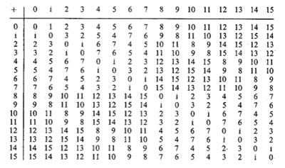
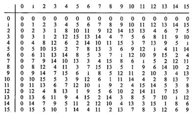
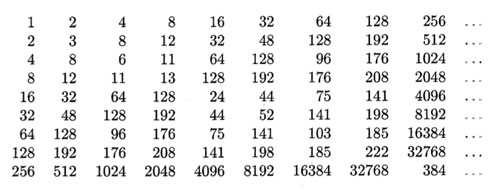
On the natural numbers the Conway-addition is binary addition without carrying and Conway-multiplication is defined by the properties that two different Fermat-powers $N=2^{2^i} $ multiply as they do in the natural numbers, and, Fermat-powers square to its sesquimultiple, that is $N^2=\frac{3}{2}N $. Moreover, all natural numbers smaller than $N=2^{2^{i}} $ form a finite field $\mathbb{F}_{2^{2^i}} $. Using distributivity, one can write down a multiplication table for all 2-powers.

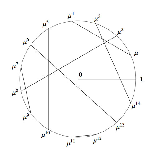
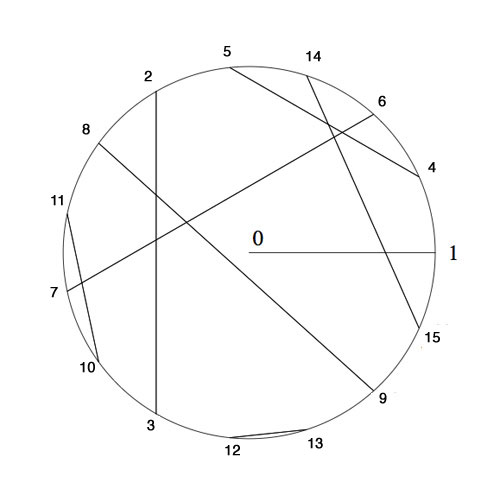
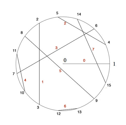
The Knight-seating problems asks for a consistent placing of n-th Knight $K_n $ at an odd root of unity, compatible with the two different realizations of $\overline{\mathbb{F}_2} $. Last time, we were able to place the first 15 Knights as below, and asked where you would seat $K_{16} $

$K_4 $ was placed at $e^{2\pi i/15} $ as 4 was the smallest number generating the ‘Fermat’-field $\mathbb{F}_{2^{2^2}} $ (with multiplicative group of order 15) subject to the compatibility relation with the generator 2 of the smaller Fermat-field $\mathbb{F}_2 $ (with group of order 15) that $4^5=2 $.

To include the next Fermat-field $\mathbb{F}_{2^{2^3}} $ (with multiplicative group of order 255) consistently, we need to find the smallest number n generating the multiplicative group and satisfying the compatibility condition $n^{17}=4 $. Let’s first concentrate on finding the smallest generator : as 2 is a generator for 1st Fermat-field $\mathbb{F}_{2^{2^1}} $ and 4 a generator for the 2-nd Fermat-field $\mathbb{F}_{2^{2^2}} $ a natural conjecture might be that 16 is a generator for the 3-rd Fermat-field $\mathbb{F}_{2^{2^3}} $ and, more generally, that $2^{2^i} $ would be a generator for the next field $\mathbb{F}_{2^{2^{i+1}}} $.

However, an “exercise” in the 1978-paper by Hendrik Lenstra Nim multiplication asks : “Prove that $2^{2^i} $ is a primitive root in the field $\mathbb{F}_{2^{2^{i+1}}} $ if and only if i=0 or 1.”

I’ve struggled with several of the ‘exercises’ in Lenstra’s paper to the extend I feared Alzheimer was setting in, only to find out, after taking pen and paper and spending a considerable amount of time calculating, that they are indeed merely exercises, when looked at properly… (Spoiler-warning : stop reading now if you want to go through this exercise yourself).

In the picture above I’ve added in red the number $x(x+1)=x^2+1 $ to each of the involutions. Clearly, for each pair these numbers are all distinct and we see that for the indicated pairing they make up all numbers strictly less than 8.

By Conway’s simplicity rules (or by checking) the pair (16,17) gives the number 8. In other words, the equation
$x^2+x+8 $ is an irreducible polynomial over $\mathbb{F}_{16} $ having as its roots in $\mathbb{F}_{256} $ the numbers 16 and 17. But then, 16 and 17 are conjugated under the Galois-involution (the Frobenius $y \mapsto y^{16} $). That is, we have $16^{16}=17 $ and $17^{16}=16 $ and hence $16^{17}=8 $. Now, use the multiplication table in $\mathbb{F}_{16} $ given in the previous post (or compute!) to see that 8 is of order 5 (and NOT a generator). As a consequence, the multiplicative order of 16 is 5×17=85 and so 16 cannot be a generator in $\mathbb{F}_{256} $.
For general i one uses the fact that $2^{2^i} $ and $2^{2^i}+1 $ are the roots of the polynomial $x^2+x+\prod_{j<i} 2^{2^j} $ over $\mathbb{F}_{2^{2^i}} $ and argues as before.

Right, but then what is the minimal generator satisfying $n^{17}=4 $? By computing we see that the pairings of all numbers in the range 16…31 give us all numbers in the range 8…15 and by the above argument this implies that the 17-th powers of all numbers smaller than 32 must be different from 4. But then, the smallest candidate is 32 and one verifies that indeed $32^{17}=4 $ (use the multiplication table given before).

Hence, we must place Knight $K_{32} $ at root $e^{2 \pi i/255} $ and place the other Knights prior to the 256-th at the corresponding power of 32. I forgot the argument I used to find-by-hand the requested place for Knight 16, but one can verify that $32^{171}=16 $ so we seat $K_{16} $ at root $e^{342 \pi i/255} $.

But what about Knight $K_{256} $? Well, by this time I was quite good at squaring and binary representations of integers, but also rather tired, and decided to leave that task to the computer.

If we denote Nim-addition and multiplication by $\oplus $ and $\otimes $, then Conway’s simplicity results in ONAG establish a field-isomorphism between $~(\mathbb{N},\oplus,\otimes) $ and the field $\mathbb{F}_2(x_0,x_1,x_2,\ldots ) $ where the $x_i $ satisfy the Artin-Schreier equations

$x_i^2+x_i+\prod_{j < i} x_j = 0 $

and the i-th Fermat-field $\mathbb{F}_{2^{2^i}} $ corresponds to $\mathbb{F}_2(x_0,x_1,\ldots,x_{i-1}) $. The correspondence between numbers and elements from these fields is given by taking $x_i \mapsto 2^{2^i} $. But then, wecan write every 2-power as a product of the $x_i $ and use the binary representation of numbers to perform all Nim-calculations with numbers in these fields.

Therefore, a quick and dirty way (and by no means the most efficient) to do Nim-calculations in the next Fermat-field consisting of all numbers smaller than 65536, is to use sage and set up the field $\mathbb{F}_2(x_0,x_1,x_2,x_3) $ by

R.< x,y,z,t > =GF(2)[]
S.< a,b,c,d >=R.quotient((x^2+x+1,y^2+y+x,z^2+z+x*y,t^2+t+x*y*z))

To find the smallest number generating the multiplicative group and satisfying the additional compatibility condition $n^{257}=32 $ we have to find the smallest binary number $i_1i_2 \ldots i_{16} $ (larger than 255) satisfying

(i1*a*b*c*t+i2*b*c*t+i3*a*c*t+i4*c*t+i5*a*b*t+i6*b*t+
i7*a*t+i8*t+i9*a*b*c+i10*b*c+i11*a*c+i12*c+i13*a*b+
i14*b+i15*a+i16)^257=a*c

It takes a 2.4GHz 2Gb-RAM MacBook not that long to decide that the requested generator is 1051 (killing another optimistic conjecture that these generators might be 2-powers). So, we seat Knight
$K_{1051} $ at root $e^{2 \pi i/65535} $ and can then arrange seatings for all Knight queued up until we reach the 65536-th! In particular, the first Knight we couldn’t place before, that is Knight $K_{256} $, will be seated at root $e^{65826 \pi i/65535} $.

If you’re lucky enough to own a computer with more RAM, or have the patience to make the search more efficient and get the seating arrangement for the next Fermat-field, please drop a comment.

I’ll leave you with another Lenstra-exercise which shouldn’t be too difficult for you to solve now : “Prove that $x^3=2^{2^i} $ has three solutions in $\mathbb{N} $ for each $i \geq 2 $.”

2 Comments

big Witt vectors for everyone (1/2)

Published February 2, 2010 by lievenlb

Next time you visit your math-library, please have a look whether these books are still on the shelves : Michiel Hazewinkel‘s Formal groups and applications, William Fulton’s and Serge Lange’s Riemann-Roch algebra and Donald Knutson’s lambda-rings and the representation theory of the symmetric group.

I wouldn’t be surprised if one or more of these books are borrowed out, probably all of them to the same person. I’m afraid I’m that person in Antwerp…

Lately, there’s been a renewed interest in $\lambda $-rings and the endo-functor W assigning to a commutative algebra its ring of big Witt vectors, following Borger’s new proposal for a geometry over the absolute point.

However, as Hendrik Lenstra writes in his 2002 course-notes on the subject Construction of the ring of Witt vectors : “The literature on the functor W is in a somewhat unsatisfactory state: nobody seems to have any interest in Witt vectors beyond applying them for a purpose, and they are often treated in appendices to papers devoting to something else; also, the construction usually depends on a set of implicit or unintelligible formulae. Apparently, anybody who wishes to understand Witt vectors needs to construct them personally. That is what is now happening to myself.”

Before doing a series on Borger’s paper, we’d better run through Lenstra’s elegant construction in a couple of posts. Let A be a commutative ring and consider the multiplicative group of all ‘one-power series’ over it $\Lambda(A)=1+t A[[t]] $. Our aim is to define a commutative ring structure on $\Lambda(A) $ taking as its ADDITION the MULTIPLICATION of power series.

That is, if $u(t),v(t) \in \Lambda(A) $, then we define our addition $u(t) \oplus v(t) = u(t) \times v(t) $. This may be slightly confusing as the ZERO-element in $\Lambda(A),\oplus $ will then turn be the constant power series 1…

We are now going to define a multiplication $\otimes $ on $\Lambda(A) $ which is distributively with respect to $\oplus $ and turns $\Lambda(A) $ into a commutative ring with ONE-element the series $~(1-t)^{-1}=1+t+t^2+t^3+\ldots $.

We will do this inductively, so consider $\Lambda_n(A) $ the (classes of) one-power series truncated at term n, that is, the kernel of the natural augmentation map between the multiplicative group-units $~A[t]/(t^{n+1})^* \rightarrow A^* $.
Again, taking multiplication in $A[t]/(t^{n+1}) $ as a new addition rule $\oplus $, we see that $~(\Lambda_n(A),\oplus) $ is an Abelian group, whence a $\mathbb{Z} $-module.

For all elements $a \in A $ we have a scaling operator $\phi_a $ (sending $t \rightarrow at $) which is an A-ring endomorphism of $A[t]/(t^{n+1}) $, in particular multiplicative wrt. $\times $. But then, $\phi_a $ is an additive endomorphism of $~(\Lambda_n(A),\oplus) $, so is an element of the endomorphism-RING $End_{\mathbb{Z}}(\Lambda_n(A)) $. Because composition (being the multiplication in this endomorphism ring) of scaling operators is clearly commutative ($\phi_a \circ \phi_b = \phi_{ab} $) we can define a commutative RING $E $ being the subring of $End_{\mathbb{Z}}(\Lambda_n(A)) $ generated by the operators $\phi_a $.

The action turns $~(\Lambda_n(A),\oplus) $ into an E-module and we define an E-module morphism $E \rightarrow \Lambda_n(A) $ by $\phi_a \mapsto \phi_a((1-t)^{-1}) = (1-at)^{-a} $.

All of this looks pretty harmless, but the upshot is that we have now equipped the image of this E-module morphism, say $L_n(A) $ (which is the additive subgroup of $~(\Lambda_n(A),\oplus) $ generated by the elements $~(1-at)^{-1} $) with a commutative multiplication $\otimes $ induced by the rule $~(1-at)^{-1} \otimes (1-bt)^{-1} = (1-abt)^{-1} $.

Explicitly, $L_n(A) $ is the set of one-truncated polynomials $u(t) $ with coefficients in $A $ such that one can find elements $a_1,\ldots,a_k \in A $ such that $u(t) \equiv (1-a_1t)^{-1} \times \ldots \times (1-a_k)^{-1}~mod~t^{n+1} $. We multiply $u(t) $ with another such truncated one-polynomial $v(t) $ (taking elements $b_1,b_2,\ldots,b_l \in A $) via

$u(t) \otimes v(t) = ((1-a_1t)^{-1} \oplus \ldots \oplus (1-a_k)^{-1}) \otimes ((1-b_1t)^{-1} \oplus \ldots \oplus (1-b_l)^{-1}) $

and using distributivity and the multiplication rule this gives the element $\prod_{i,j} (1-a_ib_jt)^{-1}~mod~t^{n+1} \in L_n(A) $.
Being a ring-qutient of $E $ we have that $~(L_n(A),\oplus,\otimes) $ is a commutative ring, and, from the construction it is clear that $L_n $ behaves functorially.

For rings $A $ such that $L_n(A)=\Lambda_n(A) $ we are done, but in general $L_n(A) $ may be strictly smaller. The idea is to use functoriality and do the relevant calculations in a larger ring $A \subset B $ where we can multiply the two truncated one-polynomials and observe that the resulting truncated polynomial still has all its coefficients in $A $.

Here’s how we would do this over $\mathbb{Z} $ : take two irreducible one-polynomials u(t) and v(t) of degrees r resp. s smaller or equal to n. Then over the complex numbers we have
$u(t)=(1-\alpha_1t) \ldots (1-\alpha_rt) $ and $v(t)=(1-\beta_1) \ldots (1-\beta_st) $. Then, over the field $K=\mathbb{Q}(\alpha_1,\ldots,\alpha_r,\beta_1,\ldots,\beta_s) $ we have that $u(t),v(t) \in L_n(K) $ and hence we can compute their product $u(t) \otimes v(t) $ as before to be $\prod_{i,j}(1-\alpha_i\beta_jt)^{-1}~mod~t^{n+1} $. But then, all coefficients of this truncated K-polynomial are invariant under all permutations of the roots $\alpha_i $ and the roots $\beta_j $ and so is invariant under all elements of the Galois group. But then, these coefficients are algebraic numbers in $\mathbb{Q} $ whence integers. That is, $u(t) \otimes v(t) \in \Lambda_n(\mathbb{Z}) $. It should already be clear from this that the rings $\Lambda_n(\mathbb{Z}) $ contain a lot of arithmetic information!

For a general commutative ring $A $ we will copy this argument by considering a free overring $A^{(\infty)} $ (with 1 as one of the base elements) by formally adjoining roots. At level 1, consider $M_0 $ to be the set of all non-constant one-polynomials over $A $ and consider the ring

$A^{(1)} = \bigotimes_{f \in M_0} A[X]/(f) = A[X_f, f \in M_0]/(f(X_f) , f \in M_0) $

The idea being that every one-polynomial $f \in M_0 $ now has one root, namely $\alpha_f = \overline{X_f} $ in $A^{(1)} $. Further, $A^{(1)} $ is a free A-module with basis elements all $\alpha_f^i $ with $0 \leq i < deg(f) $.

Good! We now have at least one root, but we can continue this process. At level 2, $M_1 $ will be the set of all non-constant one-polynomials over $A^{(1)} $ and we use them to construct the free overring $A^{(2)} $ (which now has the property that every $f \in M_0 $ has at least two roots in $A^{(2)} $). And, again, we repeat this process and obtain in succession the rings $A^{(3)},A^{(4)},\ldots $. Finally, we define $A^{(\infty)} = \underset{\rightarrow}{lim}~A^{(i)} $ having the property that every one-polynomial over A splits entirely in linear factors over $A^{(\infty)} $.

But then, for all $u(t),v(t) \in \Lambda_n(A) $ we can compute $u(t) \otimes v(t) \in \Lambda_n(A^{(\infty)}) $. Remains to show that the resulting truncated one-polynomial has all its entries in A. The ring $A^{(\infty)} \otimes_A A^{(\infty)} $ contains two copies of $A^{(\infty)} $ namely $A^{(\infty)} \otimes 1 $ and $1 \otimes A^{(\infty)} $ and the intersection of these two rings in exactly $A $ (here we use the freeness property and the additional fact that 1 is one of the base elements). But then, by functoriality of $L_n $, the element
$u(t) \otimes v(t) \in L_n(A^{(\infty)} \otimes_A A^{(\infty)}) $ lies in the intersection $\Lambda_n(A^{(\infty)} \otimes 1) \cap \Lambda_n(1 \otimes A^{(\infty)})=\Lambda_n(A) $. Done!

Hence, we have endo-functors $\Lambda_n $ in the category of all commutative rings, for every number n. Reviewing the construction of $L_n $ one observes that there are natural transformations $L_{n+1} \rightarrow L_n $ and therefore also natural transformations $\Lambda_{n+1} \rightarrow \Lambda_n $. Taking the inverse limits $\Lambda(A) = \underset{\leftarrow}{lim} \Lambda_n(A) $ we therefore have the ‘one-power series’ endo-functor
$\Lambda~:~\mathbf{comm} \rightarrow \mathbf{comm} $
which is ‘almost’ the functor W of big Witt vectors. Next time we’ll take you through the identification using ‘ghost variables’ and how the functor $\Lambda $ can be used to define the category of $\lambda $-rings.

One Comment

The odd knights of the round table

Published January 28, 2010 by lievenlb

Here’s a tiny problem illustrating our limited knowledge of finite fields : “Imagine an infinite queue of Knights ${ K_1,K_2,K_3,\ldots } $, waiting to be seated at the unit-circular table. The master of ceremony (that is, you) must give Knights $K_a $ and $K_b $ a place at an odd root of unity, say $\omega_a $ and $\omega_b $, such that the seat at the odd root of unity $\omega_a \times \omega_b $ must be given to the Knight $K_{a \otimes b} $, where $a \otimes b $ is the Nim-multiplication of $a $ and $b $. Which place would you offer to Knight $K_{16} $, or Knight $K_n $, or, if you’re into ordinals, Knight $K_{\omega} $?”

What does this have to do with finite fields? Well, consider the simplest of all finite field $\mathbb{F}_2 = { 0,1 } $ and consider its algebraic closure $\overline{\mathbb{F}_2} $. Last year, we’ve run a series starting here, identifying the field $\overline{\mathbb{F}_2} $, following John H. Conway in ONAG, with the set of all ordinals smaller than $\omega^{\omega^{\omega}} $, given the Nim addition and multiplication. I know that ordinal numbers may be intimidating at first, so let’s just restrict to ordinary natural numbers for now. The Nim-addition of two numbers $n \oplus m $ can be calculated by writing the numbers n and m in binary form and add them without carrying. For example, $9 \oplus 1 = 1001+1 = 1000 = 8 $. Nim-multiplication is slightly more complicated and is best expressed using the so-called Fermat-powers $F_n = 2^{2^n} $. We then demand that $F_n \otimes m = F_n \times m $ whenever $m < F_n $ and $F_n \otimes F_n = \frac{3}{2}F_n $. Distributivity wrt. $\oplus $ can then be used to calculate arbitrary Nim-products. For example, $8 \otimes 3 = (4 \otimes 2) \otimes (2 \oplus 1) = (4 \otimes 3) \oplus (4 \otimes 2) = 12 \oplus 8 = 4 $. Conway’s remarkable result asserts that the ordinal numbers, equipped with Nim addition and multiplication, form an algebraically closed field of characteristic two. The closure $\overline{\mathbb{F}_2} $ is identified with the subfield of all ordinals smaller than $\omega^{\omega^{\omega}} $. For those of you who don’t feel like going transfinite, the subfield $~(\mathbb{N},\oplus,\otimes) $ is identified with the quadratic closure of $\mathbb{F}_2 $.

The connection between $\overline{\mathbb{F}_2} $ and the odd roots of unity has been advocated by Alain Connes in his talk before a general public at the IHES : “L’ange de la géométrie, le diable de l’algèbre et le corps à un élément” (the angel of geometry, the devil of algebra and the field with one element). He describes its content briefly in this YouTube-video

At first it was unclear to me which ‘coupling-problem’ Alain meant, but this has been clarified in his paper together with Caterina Consani Characteristic one, entropy and the absolute point. The non-zero elements of $\overline{\mathbb{F}_2} $ can be identified with the set of all odd roots of unity. For, if x is such a unit, it belongs to a finite subfield of the form $\mathbb{F}_{2^n} $ for some n, and, as the group of units of any finite field is cyclic, x is an element of order $2^n-1 $. Hence, $\mathbb{F}_{2^n}- { 0 } $ can be identified with the set of $2^n-1 $-roots of unity, with $e^{2 \pi i/n} $ corresponding to a generator of the unit-group. So, all elements of $\overline{\mathbb{F}_2} $ correspond to an odd root of unity. The observation that we get indeed all odd roots of unity may take you a couple of seconds (( If m is odd, then (2,m)=1 and so 2 is a unit in the finite cyclic group $~(\mathbb{Z}/m\mathbb{Z})^* $ whence $2^n = 1 (mod~m) $, so the m-roots of unity lie within those of order $2^n-1 $ )).

Assuming we succeed in fixing a one-to-one correspondence between the non-zero elements of $\overline{\mathbb{F}_2} $ and the odd roots of unity $\mu_{odd} $ respecting multiplication, how can we recover the addition on $\overline{\mathbb{F}_2} $? Well, here’s Alain’s coupling function, he ties up an element x of the algebraic closure to the element s(x)=x+1 (and as we are in characteristic two, this is an involution, so also the element tied up to x+1 is s(x+1)=(x+1)+1=x. The clue being that multiplication together with the coupling map s allows us to compute any sum of two elements as $x+y=x \times s(\frac{y}{x}) = x \times (\frac{y}{x}+1) $.
For example, all information about the finite field $\mathbb{F}_{2^4} $ is encoded in this identification with the 15-th roots of unity, together with the pairing s depicted as

Okay, we now have two identifications of the algebraic closure $\overline{\mathbb{F}_2} $ : the smaller ordinals equipped with Nim addition and Nim multiplication and the odd roots of unity with complex-multiplication and the Connes-coupling s. The question we started from asks for a general recipe to identify these two approaches.

To those of you who are convinced that finite fields (LOL, even characteristic two!) are objects far too trivial to bother thinking about : as far as I know, NOBODY knows how to do this explicitly, even restricting the ordinals to merely the natural numbers!

Please feel challenged! To get you started, I’ll show you how to place the first 15 Knights and give you a procedure (though far from explicit) to continue. Here’s the Nim-picture compatible with that above

To verify this, and to illustrate the general strategy, I’d better hand you the Nim-tables of the first 16 numbers. Here they are

It is known that the finite subfields of $~(\mathbb{N},\oplus,\otimes) $ are precisely the sets of numbers smaller than the Fermat-powers $F_n $. So, the first one is all numbers smaller than $F_1=4 $ (check!). The smallest generator of the multiplicative group (of order 3) is 2, so we take this to correspond to the unit-root $e^{2 \pi i/3} $. The next subfield are all numbers smaller than $F_2 = 16 $ and its multiplicative group has order 15. Now, choose the smallest integer k which generates this group, compatible with the condition that $k^{\otimes 5}=2 $. Verify that this number is 4 and that this forces the identification and coupling given above.

The next finite subfield would consist of all natural numbers smaller than $F_3=256 $. Hence, in this field we are looking for the smallest number k generating the multiplicative group of order 255 satisfying the extra condition that $k^{\otimes 17}=4 $ which would fix an identification at that level. Then, the next level would be all numbers smaller than $F_4=65536 $ and again we would like to find the smallest number generating the multiplicative group and such that the appropriate power is equal to the aforementioned k, etc. etc.

Can you give explicit (even inductive) formulae to achieve this? I guess even the problem of placing Knight 16 will give you a couple of hours to think about… (to be continued).