Tag: Conway

a monstrous unimodular lattice

Published April 30, 2021 by lievenlb

An integral $n$-dimensional lattice $L$ is the set of all integral linear combinations
\[
L = \mathbb{Z} \lambda_1 \oplus \dots \oplus \mathbb{Z} \lambda_n \]
of base vectors $\{ \lambda_1,\dots,\lambda_n \}$ of $\mathbb{R}^n$, equipped with the usual (positive definite) inner product, satisfying
\[
(\lambda, \mu ) \in \mathbb{Z} \quad \text{for all $\lambda,\mu \in \mathbb{Z}$.} \]
But then, $L$ is contained in its dual lattice $L^* = Hom_{\mathbb{Z}}(L,\mathbb{Z})$, and if $L = L^*$ we say that $L$ is unimodular.

If all $(\lambda,\lambda) \in 2 \mathbb{Z}$, we say that $L$ is an even lattice. Even unimodular lattices (such as the $E_8$-lattice or the $24$ Niemeier lattices) are wonderful objects, but they can only live in dimensions $n$ which are multiples of $8$.

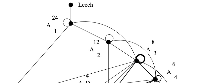
Just like the Conway group $Co_0 = .0$ is the group of rotations of the Leech lattice $\Lambda$, one might ask whether there is a very special lattice on which the Monster group $\mathbb{M}$ acts faithfully by rotations. If such a lattice exists, it must live in dimension at least $196883$.

Simon Norton (1952-2019) – Photo Credit

A first hint of such a lattice is in Conway’s original paper A simple construction for the Fischer-Griess monster group (but not in the corresponding chapter 29 of SPLAG).

Conway writes that Simon Norton showed ‘by a very simple computations that does not even require knowledge of the conjugacy classes, that any $198883$-dimensional representation of the Monster must support an invariant algebra’, which, after adding an identity element $1$, we now know as the $196884$-dimensional Griess algebra.

Further, on page 529, Conway writes:

Norton has shown that the lattice $L$ spanned by vectors of the form $1,t,t \ast t’$, where $t$ and $t’$ are transposition vectors, is closed under the algebra multiplication and integral with respect to the doubled inner product $2(u,v)$. The dual quotient $L^*/L$ is cyclic of order some power of $4$, and we believe that in fact $L$ is unimodular.

Here, transposition vectors correspond to transpositions in $\mathbb{M}$, that is, elements of conjugacy class $2A$.

I only learned about this lattice yesterday via the MathOverflow-post A lattice with Monster group symmetries by Adam P. Goucher.

In his post, Adam considers the $196883$-dimensional lattice $L’ = L \cap 1^{\perp}$ (which has $\mathbb{M}$ as its rotation symmetry group), and asks for the minimal norm (squared) of a lattice point, which he believes is $448$, and for the number of minimal vectors in the lattice, which might be
\[
2639459181687194563957260000000 = 9723946114200918600 \times 27143910000 \]
the number of oriented arcs in the Monster graph.

Here, the Monster graph has as its vertices the elements of $\mathbb{M}$ in conjugacy class $2A$ (which has $9723946114200918600$ elements) and with an edge between two vertices if their product in $\mathbb{M}$ again belongs to class $2A$, so the valency of the graph must be $27143910000$, as explained in that old post the monster graph and McKay’s observation.

When I asked Adam whether he had more information about his lattice, he kindly informed me that Borcherds told him that the Norton lattice $L$ didn’t turn out to be unimodular after all, but that a unimodular lattice with monstrous symmetry had been constructed by Scott Carnahan in the paper A Self-Dual Integral Form of the Moonshine Module.

Scott Carnahan – Photo Credit

The major steps (or better, the little bit of it I could grasp in this short time) in the construction of this unimodular $196884$-dimensional monstrous lattice might put a smile on your face if you are an affine scheme aficionado.

Already in his paper Vertex algebras, Kac-Moody algebras, and the Monster, Richard Borcherds described an integral form of any lattice vertex algebra. We’ll be interested in the lattice vertex algebra $V_{\Lambda}$ constructed from the Leech lattice $\Lambda$ and call its integral form $(V_{\Lambda})_{\mathbb{Z}}$.

One constructs the Moonshine module $V^{\sharp}$ from $V_{\Lambda}$ by a process called ‘cyclic orbifolding’, a generalisation of the original construction by Frenkel, Lepowsky and Meurman. In fact, there are now no less than 51 constructions of the moonshine module.

One starts with a fixed point free rotation $r_p$ of $\Lambda$ in $Co_0$ of prime order $p \in \{ 2,3,5,7,13 \}$, which one can lift to an automorphism $g_p$ of the vertex algebra $V_{\Lambda}$ of order $p$ giving an isomorphism $V_{\Lambda}/g_p \simeq V^{\sharp}$ of vertex operator algebras over $\mathbb{C}$.

For two distinct primes $p,p’ \in \{ 2,3,5,7,13 \}$ if $Co_0$ has an element of order $p.p’$ one can find one such $r_{pp’}$ such that $r_{pp’}^p=r_{p’}$ and $r_{pp’}^{p’}=r_p$, and one can lift $r_{pp’}$ to an automorphism $g_{pp’}$ of $V_{\Lambda}$ such that $V_{\Lambda}/g_{pp’} \simeq V_{\Lambda}$ as vertex operator algebras over $\mathbb{C}$.

Problem is that these lifts of automorphisms and the isomorphisms are not compatible with the integral form $(V_{\Lambda})_{\mathbb{Z}}$ of $V_{\Lambda}$, but ‘essentially’, they can be performed on
\[
(V_{\Lambda})_{\mathbb{Z}} \otimes_{\mathbb{Z}} \mathbb{Z}[\frac{1}{pp’},\zeta_{2pp’}] \]
where $\zeta_{2pp’}$ is a primitive $2pp’$-th root of unity. These then give a $\mathbb{Z}[\tfrac{1}{pp’},\zeta_{2pp’}]$-form on $V^{\sharp}$.

Next, one uses a lot of subgroup information about $\mathbb{M}$ to prove that these $\mathbb{Z}[\tfrac{1}{pp’},\zeta_{2pp’}]$-forms of $V^{\sharp}$ have $\mathbb{M}$ as their automorphism group.

Then, using all his for different triples in $\{ 2,3,5,7,13 \}$ one can glue and use faithfully flat descent to get an integral form $V^{\sharp}_{\mathbb{Z}}$ of the moonshine module with monstrous symmetry and such that the inner product on $V^{\sharp}_{\mathbb{Z}}$ is positive definite.

Finally, one looks at the weight $2$ subspace of $V^{\sharp}_{\mathbb{Z}}$ which gives us ~~our~~ Carnahan’s $196884$-dimensional unimodular lattice with monstrous symmetry!

Beautiful as this is, I guess it will be a heck of a project to deduce even the simplest of facts about this wonderful lattice from running through this construction.

For example, what is the minimal length of vectors? What is the number of minimal length vectors? And so on. All info you might have is very welcome.

One Comment

The Leech lattice neighbour

Published March 23, 2021 by lievenlb

Here’s the upper part of Kneser‘s neighbourhood graph of the Niemeier lattices:

The Leech lattice has a unique neighbour, that is, among the $23$ remaining Niemeier lattices there is a unique one, $(A_1^{24})^+$, sharing an index two sub-lattice with the Leech.

How would you try to construct $(A_1^{24})^+$, an even unimodular lattice having the same roots as $A_1^{24}$?

The root lattice $A_1$ is $\sqrt{2} \mathbb{Z}$. It has two roots $\pm \sqrt{2}$, determinant $2$, its dual lattice is $A_1^* = \tfrac{1}{\sqrt{2}} \mathbb{Z}$ and we have $A_1^*/A_1 \simeq C_2 \simeq \mathbb{F}_2$.

Thus, $A_1^{24}= \sqrt{2} \mathbb{Z}^{\oplus 24}$ has $48$ roots, determinant $2^{24}$, its dual lattice is $(A_1^{24})^* = \tfrac{1}{\sqrt{2}} \mathbb{Z}^{\oplus 24}$ and the quotient group $(A_1^{24})^*/A_1^{24}$ is $C_2^{24}$ isomorphic to the additive subgroup of $\mathbb{F}_2^{\oplus 24}$.

A larger lattice $A_1^{24} \subseteq L$ of index $k$ gives for the dual lattices an extension $L^* \subseteq (A_1^{24})^*$, also of index $k$. If $L$ were unimodular, then the index has to be $2^{12}$ because we have the situation
\[
A_1^{24} \subseteq L = L^* \subseteq (A_1^{24})^* \]
So, Kneser’s glue vectors form a $12$-dimensional subspace $\mathcal{C}$ in $\mathbb{F}_2^{\oplus 24}$, that is,
\[
L = \mathcal{C} \underset{\mathbb{F}_2}{\times} (A_1^{24})^* = \{ \tfrac{1}{\sqrt{2}} \vec{v} ~|~\vec{v} \in \mathbb{Z}^{\oplus 24},~v=\vec{v}~mod~2 \in \mathcal{C} \} \]
Because $L = L^*$, the linear code $\mathcal{C}$ must be self-dual meaning that $v.w = 0$ (in $\mathbb{F}_2$) for all $v,w \in \mathcal{C}$. Further, we want that the roots of $A_1^{24}$ and $L$ are the same, so the minimal number of non-zero coordinates in $v \in \mathcal{C}$ must be $8$.

That is, $\mathcal{C}$ must be a self-dual binary code of length $24$ with Hamming distance $8$.

Marcel Golay (1902-1989) – Photo Credit

We now know that there is a unique such code, the (extended) binary Golay code, $\mathcal{C}_{24}$, which has

one vector of weight $0$
$759$ vectors of weight $8$ (called ‘octads’)
$2576$ vectors of weight $12$ (called ‘dodecads’)
$759$ vectors of weight $16$
one vector of weight $24$

The $759$ octads form a Steiner system $S(5,8,24)$ (that is, for any $5$-subset $S$ of the $24$-coordinates there is a unique octad having its non-zero coordinates containing $S$).

Witt constructed a Steiner system $S(5,8,24)$ in his 1938 paper “Die $5$-fach transitiven Gruppen von Mathieu”, so it is not unthinkable that he checked the subspace of $\mathbb{F}_2^{\oplus 24}$ spanned by his $759$ octads to be $12$-dimensional and self-dual, thereby constructing the Niemeier-lattice $(A_1^{24})^+$ on that sunday in 1940.

John Conway classified all nine self-dual codes of length $24$ in which the weight
of every codeword is a multiple of $4$. Each one of these codes $\mathcal{C}$ gives a Niemeier lattice $\mathcal{C} \underset{\mathbb{F}_2}{\times} (A_1^{24})^*$, all but one of them having more roots than $A_1^{24}$.

Vera Pless and Neil Sloan classified all $26$ binary self-dual codes of length $24$.

Penrose’s aperiodic tilings

Published March 9, 2021 by lievenlb

Around 1975 Sir Roger Penrose discovered his aperiodic P2 tilings of the plane, using only two puzzle pieces: Kites (K) and Darts (D)

The inner angles of these pieces are all multiples of $36^o = \tfrac{180^o}{5}$, the short edges have length $1$, and the long edges have length $\tau = \tfrac{1+\sqrt{5}}{2}$, the golden ratio. These pieces must be joined together so that the colours match up (if we do not use this rule it is easy to get periodic tilings with these two pieces).

There is plenty of excellent online material available:

The two original Martin Gardner Scientific American articles on Penrose tiles have been made available by the MAA, and were reprinted in “Penrose Tiles to Trapdoor Ciphers”. They contain most of Conway’s early discoveries about these tilings, but without proofs.
A JavaScript application by Kevin Bertman to play around with these tilings. You can deflate and inflate tilings, find forced tiles and much more. Beneath the app-window there’s a detailed explanation of all the basics, including inflation and deflation of the P2-tiles, the seven types of local vertex configurations (naming by Conway, of course),

proofs of aperiodicity (similar to the one for Conway’s musical sequences), that every tile lies within an ace (similar to the LSL-subword in musical sequences) with application to local isomorphism (again similar to the $1$-dimensional case).
Course notes of an Oxford masterclass in geometry Lectures on Penrose tilings by Alexander Ritter, again with proofs of all of the above and a discussion about the Cartwheel tilings (similar to that in the post on musical sequences), giving an algorithm to decide whether or not a partial tiling can be extended to the entire plane, or not.

There’s no point copying this material here. Rather, I’d like to use some time in this GoV series of posts to talk about de Bruijn’s pentagrid results. For this reason, I now need to make the connection with Penrose’s ‘other’ tilings, the P3 tiles of ‘thin’ and ‘thick’ rhombi (sometimes called ‘skinny’ and ‘fat’ rhombi).

Every Penrose P2-tiling can be turned into a P3-rhombic tiling, and conversely.

From kites and darts to rhombi: divide every kite in two halves along its line of reflection. Then combine darts and half-kites into rhombi where a fat rhombus consists of a dart and two half-kites, joined at a long edge, and a skinny rhombus is made of two half-kites, joined at a short edge. This can always be done preserving the gluing conditions. It suffices to verify this for the deflated kite and dart (on the left below) and we see that the matching colour-conditions are those of the rhombi.

From rhombi to kites and darts: divide every fat rhombus into a dart (placed at the red acute angle) and two half-kites, joined at a long edge, and divide every skinny rhombus into two half-kites along its short diagonal.

All results holding for Kites and Darts tilings have therefore their versions for Rhombic tilings. For example, we have rhombic deflation and inflation rules

A Rhombic tiling can be seen as an intermediate step in the inflation process of a Penrose tiling $P$. Start by dividing all kites in two halves along their long diagonal and all darts in two halves along their short diagonal (the purple lines below).

If we consider all original black lines together with the new purple ones, we get a tiling of the plane by triangles and we call this the $A$-tiling. There are two triangles, s small triangle $S_A$ (the whiter ones, with two small edges ofd length $1$ and one edge of length $\tau$) and a large triangle $L_A$ (the greyer ones, with two edges of length $\tau$ and one edge of length $1$).

Next, we remove the black lines joining an $S_A$-triangle with an $L_A$-triangle, and get another tiling with triangles, the $B$-tiling, with two pieces, a large triangle $L_B$ with two sides of length $\tau$ and one side of length $1+\tau$ (the white ones) (the union of an $L_A$ and a $S_A$), and a small triangle $S_B$ which has the same form as $L_A$ (the greyer ones). If we now join two white triangles $L_B$ along their common longer edge, and two greyer triangles $S_B$ along their common smaller edge, we obtain the Rhombic tiling $R$ corresponding to $P$.

We can repeat this process starting with the Rhombic tiling $R$. We divide all fat rhombi in two along their long diagonals, and the skinny rhombi in two along their short diagonals (the purple lines). We obtain a tiling of the plane by triangles, which is of course just the $B$-tiling above.

Remove the edge joining a small $S_B$ with a large $L_B$ triangle, then we get a new tiling by triangles, the $\tau A$-tiling consisting of large triangles $L_{\tau A}$ (the white ones) with two long edges of length $1+\tau$ and one short edge of length $\tau$ (note that $L_{\tau A}$ is $\tau$ times the triangle $L_A$), and a smaller one $S_{\tau A}$ (the grey ones) having two short edges of length $\tau$ and one long edge of length $1+\tau$ (again $S_{\tau A}$ is $\tau$ times the triangle $S_A$). If we join two $L_{\tau A}$-triangles sharing a common long edge we obtain a Kite ($\tau$-times larger than the original Kite) and if we joint two $S_{\tau A}$-triangles along their common small edge we get a Dart ($\tau$ times larger than the original Dart). The Penrose tiling we obtain is the inflation $inf(P)$ of the original $P$.

If we repeat the whole procedure starting from $inf(P)$ instead of $P$ we get, in turn, triangle tilings of the plane, subsequently the $\tau B$-tiling, the $\tau^2 A$-tiling, the $\tau^2 B$-tiling and so on, the triangles in a $\tau^n A$-tiling being of size $\tau^2$-times those of the $A$-tiling, and those in the $\tau^n B$-tiling $\tau^n$-times as large as those of the $B$-tiling.

The upshot of this is that we can associate to a Penrose tiling $P$ of the plane a sequence of $0$’s and $1$’s. Starting from $P$ we have an infinite sequence of associated triangle tilings
\[
A,~B,~\tau A,~\tau B,~\tau^2 A, \dots,~\tau^n A,~\tau^n B,~\tau^{n+1} A, \dots \]
with larger and larger triangle tiles. Let $p$ be a point of the plane lying in the interior of an $A$-tile, then we define its index sequence
\[
i(P,p) = (x_0,x_1,x_2,\dots ) \quad x_{2n} = \begin{cases} 0~\text{if $p \in L_{\tau^n A}$} \\ 1~\text{if $p \in S_{\tau^n A}$} \end{cases}~ x_{2n+1} = \begin{cases} 0~\text{if $p \in L_{\tau^n B}$} \\ 1~\text{if $p \in S_{\tau^n B}$} \end{cases} \]
That is, $x_0=1$ if $p$ lies in a small triangle of the $A$-tiling and $x_0=1$ if it lies in a large triangle, $x_1=1$ if $p$ lies in a small triangle of the $B$-tiling and is $0$ if it lies in a large $B$-triangle, and so on.

The beauty of this is that every infinite sequence $(x_0,x_1,x_2,\dots )$ whose terms are $0$ or $1$, and in which no two consecutive terms are equal to $1$, is the index sequence $i(P,p)$ of some Penrose tiling $P$ in some point $p$ of the plane.

From the construction of the sequence of triangle-tilings it follows that a small triangle is part of a large triangle in the next tiling. For this reason an index sequence can never have two consecutive ones. An index sequence gives explicit instructions as to how the Penrose tiling is constructed. In each step add a large or small triangle as to fit the sequence, together with the matching triangle (the other half of a Penrose or Rhombic tile). Next, look at the patches $P_i$ of Kites and Darts (in the $\tau^i A$ tiling), for $i=0,1,\dots$, then $P_{i-k}$ is contained in the $k$-times inflated $P_i$, $i^k(P_i)$ (without rescaling), for each $i$ and all $1 \leq k \leq i$. But then, we have a concentric series of patches
\[
P_0 \subset i(P_1) \subset i^2(P_2) \subset \dots \]
filling the entire plane.

The index sequence depends on the choice of point $p$ in the plane. If $p’$ is another point, then as the triangle tiles increase is size at each step, $p$ and $p’$ will lie in the same triangle-tile at some stage, and after that moment their index sequences will be the same.

As a result, there exists an uncountable infinity of distinct Penrose tilings of the plane.

From the discussions we see that a Penrose tiling is determined by the index-sequence in any point in the plane $(x_0,x_1,\dots )$ consisting of $0$’s and $1$’s having no two consecutive $1$’s, and that another such sequence $(x’_0,x’_1,\dots )$ determines the same Penrose tilings if $x_n=x’_n$ for all $n \geq N$ for some number $N$. That is, the Penrose tiling is determined by the the equivalence class of such sequences, and it is easy to see that there are uncountably many such equivalence classes.

If you want to play a bit with Penrose tiles, you can order the P2 tiles or the P3 tiles from
Cherry Arbor Design.