Skip to content →

Tag: Brauer

the monster graph and McKay’s observation

While the verdict on a neolithic Scottish icosahedron is still open, let us recall Kostant’s group-theoretic construction of the icosahedron from its rotation-symmetry group $A_5 $.

The alternating group $A_5 $ has two conjugacy classes of order 5 elements, both consisting of exactly 12 elements. Fix one of these conjugacy classes, say $C $ and construct a graph with vertices the 12 elements of $C $ and an edge between two $u,v \in C $ if and only if the group-product $u.v \in C $ still belongs to the same conjugacy class.

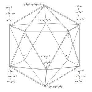
Observe that this relation is symmetric as from $u.v = w \in C $ it follows that $v.u=u^{-1}.u.v.u = u^{-1}.w.u \in C $. The graph obtained is the icosahedron, depicted on the right with vertices written as words in two adjacent elements u and v from $C $, as indicated.

Kostant writes : “Normally it is not a common practice in group theory to consider whether or not the product of two elements in a conjugacy class is again an element in that conjugacy class. However such a consideration here turns out to be quite productive.”

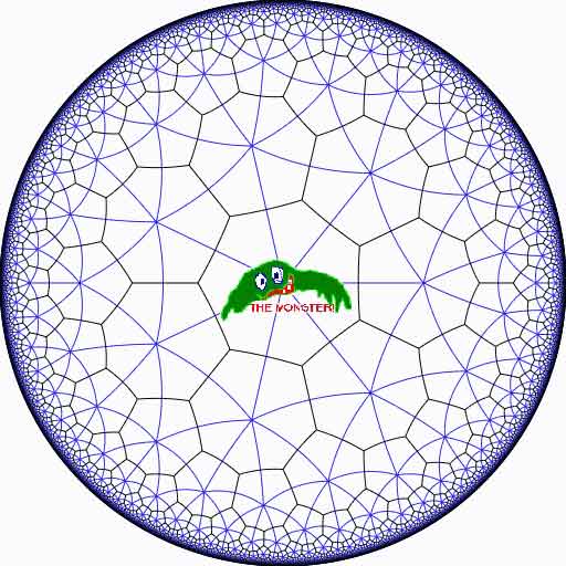
Still, similar constructions have been used in other groups as well, in particular in the study of the largest sporadic group, the monster group $\mathbb{M} $.

There is one important catch. Whereas it is quite trivial to multiply two permutations and verify whether the result is among 12 given ones, for most of us mortals it is impossible to do actual calculations in the monster. So, we’d better have an alternative way to get at the icosahedral graph using only $A_5 $-data that is also available for the monster group, such as its character table.

Let $G $ be any finite group and consider three of its conjugacy classes $C(i),C(j) $ and $C(k) $. For any element $w \in C(k) $ we can compute from the character table of $G $ the number of different products $u.v = w $ such that $u \in C(i) $ and $v \in C(j) $. This number is given by the formula

$\frac{|G|}{|C_G(g_i)||C_G(g_j)|} \sum_{\chi} \frac{\chi(g_i) \chi(g_j) \overline{\chi(g_k)}}{\chi(1)} $

where the sum is taken over all irreducible characters $\chi $ and where $g_i \in C(i),g_j \in C(j) $ and $g_k \in C(k) $. Note also that $|C_G(g)| $ is the number of $G $-elements commuting with $g $ and that this number is the order of $G $ divided by the number of elements in the conjugacy class of $g $.

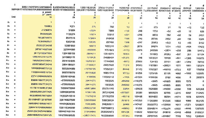
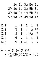
The character table of $A_5 $ is given on the left : the five columns correspond to the different conjugacy classes of elements of order resp. 1,2,3,5 and 5 and the rows are the character functions of the 5 irreducible representations of dimensions 1,3,3,4 and 5.

Let us fix the 4th conjugacy class, that is 5a, as our class $C $. By the general formula, for a fixed $w \in C $ the number of different products $u.v=w $ with $u,v \in C $ is equal to

$\frac{60}{25}(\frac{1}{1} + \frac{(\frac{1+\sqrt{5}}{2})^3}{3} + \frac{(\frac{1-\sqrt{5}}{2})^3}{3} – \frac{1}{4} + \frac{0}{5}) = \frac{60}{25}(1 + \frac{4}{3} – \frac{1}{4}) = 5 $

Because for each $x \in C $ also its inverse $x^{-1} \in C $, this can be rephrased by saying that there are exactly 5 different products $w^{-1}.u \in C $, or equivalently, that the valency of every vertex $w^{-1} \in C $ in the graph is exactly 5.

That is, our graph has 12 vertices, each with exactly 5 neighbors, and with a bit of extra work one can show it to be the icosahedral graph.

For the monster group, the Atlas tells us that it has exactly 194 irreducible representations (and hence also 194 conjugacy classes). Of these conjugacy classes, the involutions (that is the elements of order 2) are of particular importance.

There are exactly 2 conjugacy classes of involutions, usually denoted 2A and 2B. Involutions in class 2A are called “Fischer-involutions”, after Bernd Fischer, because their centralizer subgroup is an extension of Fischer’s baby Monster sporadic group.

Likewise, involutions in class 2B are usually called “Conway-involutions” because their centralizer subgroup is an extension of the largest Conway sporadic group.

Let us define the monster graph to be the graph having as its vertices the Fischer-involutions and with an edge between two of them $u,v \in 2A $ if and only if their product $u.v $ is again a Fischer-involution.

Because the centralizer subgroup is $2.\mathbb{B} $, the number of vertices is equal to $97239461142009186000 = 2^4 * 3^7 * 5^3 * 7^4 * 11 * 13^2 * 29 * 41 * 59 * 71 $.

From the general result recalled before we have that the valency in all vertices is equal and to determine it we have to use the character table of the monster and the formula. Fortunately GAP provides the function ClassMultiplicationCoefficient to do this without making errors.


gap> table:=CharacterTable("M");
CharacterTable( "M" )
gap> ClassMultiplicationCoefficient(table,2,2,2);
27143910000

Perhaps noticeable is the fact that the prime decomposition of the valency $27143910000 = 2^4 * 3^4 * 5^4 * 23 * 31 * 47 $ is symmetric in the three smallest and three largest prime factors of the baby monster order.

Robert Griess proved that one can recover the monster group $\mathbb{M} $ from the monster graph as its automorphism group!

As in the case of the icosahedral graph, the number of vertices and their common valency does not determine the monster graph uniquely. To gain more insight, we would like to know more about the sizes of minimal circuits in the graph, the number of such minimal circuits going through a fixed vertex, and so on.

Such an investigation quickly leads to a careful analysis which other elements can be obtained from products $u.v $ of two Fischer involutions $u,v \in 2A $. We are in for a major surprise, first observed by John McKay:

Printing out the number of products of two Fischer-involutions giving an element in the i-th conjugacy class of the monster,
where i runs over all 194 possible classes, we get the following string of numbers :


97239461142009186000, 27143910000, 196560, 920808, 0, 3, 1104, 4, 0, 0, 5, 0,
6, 0, 0, 0, 0, 0, 0, 0, 0, 0, 0, 0, 0, 0, 0, 0, 0, 0, 0, 0, 0, 0, 0, 0, 0, 0,
0, 0, 0, 0, 0, 0, 0, 0, 0, 0, 0, 0, 0, 0, 0, 0, 0, 0, 0, 0, 0, 0, 0, 0, 0, 0,
0, 0, 0, 0, 0, 0, 0, 0, 0, 0, 0, 0, 0, 0, 0, 0, 0, 0, 0, 0, 0, 0, 0, 0, 0, 0,
0, 0, 0, 0, 0, 0, 0, 0, 0, 0, 0, 0, 0, 0, 0, 0, 0, 0, 0, 0, 0, 0, 0, 0, 0, 0,
0, 0, 0, 0, 0, 0, 0, 0, 0, 0, 0, 0, 0, 0, 0, 0, 0, 0, 0, 0, 0, 0, 0, 0, 0, 0,
0, 0, 0, 0, 0, 0, 0, 0, 0, 0, 0, 0, 0, 0, 0, 0, 0, 0, 0, 0, 0, 0, 0, 0, 0, 0,
0, 0, 0, 0, 0, 0, 0, 0, 0, 0, 0, 0, 0, 0, 0, 0, 0, 0, 0, 0, 0, 0, 0, 0, 0, 0

That is, the elements of only 9 conjugacy classes can be written as products of two Fischer-involutions! These classes are :

  • 1A = { 1 } written in 97239461142009186000 different ways (after all involutions have order two)
  • 2A, each element of which can be written in exactly 27143910000 different ways (the valency)
  • 2B, each element of which can be written in exactly 196560 different ways. Observe that this is the kissing number of the Leech lattice leading to a permutation representation of $2.Co_1 $.
  • 3A, each element of which can be written in exactly 920808 ways. Note that this number gives a permutation representation of the maximal monster subgroup $3.Fi_{24}’ $.
  • 3C, each element of which can be written in exactly 3 ways.
  • 4A, each element of which can be written in exactly 1104 ways.
  • 4B, each element of which can be written in exactly 4 ways.
  • 5A, each element of which can be written in exactly 5 ways.
  • 6A, each element of which can be written in exactly 6 ways.

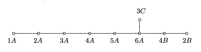
Let us forget about the actual numbers for the moment and concentrate on the orders of these 9 conjugacy classes : 1,2,2,3,3,4,4,5,6. These are precisely the components of the fundamental root of the extended Dynkin diagram $\tilde{E_8} $!

This is the content of John McKay’s E(8)-observation : there should be a precise relation between the nodes of the extended Dynkin diagram and these 9 conjugacy classes in such a way that the order of the class corresponds to the component of the fundamental root. More precisely, one conjectures the following correspondence


This is similar to the classical McKay correspondence between finite subgroups of $SU(2) $ and extended Dynkin diagrams (the binary icosahedral group corresponding to extended E(8)). In that correspondence, the nodes of the Dynkin diagram correspond to irreducible representations of the group and the edges are determined by the decompositions of tensor-products with the fundamental 2-dimensional representation.

Here, however, the nodes have to correspond to conjugacy classes (rather than representations) and we have to look for another procedure to arrive at the required edges! An exciting proposal has been put forward recently by John Duncan in his paper Arithmetic groups and the affine E8 Dynkin diagram.

It will take us a couple of posts to get there, but for now, let’s give the gist of it : monstrous moonshine gives a correspondence between conjugacy classes of the monster and certain arithmetic subgroups of $PSL_2(\mathbb{R}) $ commensurable with the modular group $\Gamma = PSL_2(\mathbb{Z}) $. The edges of the extended Dynkin E(8) diagram are then given by the configuration of the arithmetic groups corresponding to the indicated 9 conjugacy classes! (to be continued…)

Leave a Comment

the future of this blog (2)

is decided : I’ll keep maintaining this URL until new-year’s eve. At that time I’ll be blogging here for 5 years…

The few encounters I’ve had with architects, taught me this basic lesson of life : the main function of several rooms in a house changes every 5 years (due to children and yourself getting older).

So, from january 1st 2009, I’ll be moving out of here. I will leave the neverendingbooks-site intact for some time to come, so there is no need for you to start archiving it en masse, yet.

Previously I promised to reconsider this blog’s future over a short vacation, but as vacation is looking to be as illusory as the 24-dimensional monster-manifold, I spend my time throwing up ideas into thin and, it seems, extremely virtual air.

Some of you will think this is a gimmick, aiming to attract more comments (there is no post getting more responses than an imminent-end-to-this-blog-post) but then I hope to have settled this already. Neverendingbooks will die on 31st of december 2008. The only remaining issue being : do I keep on blogging or do I look for another time-consumer such as growing tomatoes or, more probably, collecting single malts…

For reasons I’ve stated before, I can see little future in anything but a conceptual-, group- blog. The first part I can deal with, but for the second I’ll be relying on others. So, all I can do is offer formats hoping that some of you are willing to take the jump and try it out together.

Such as in the bloomsday-post where I sketched the BistroMath blog-concept. Perhaps you thought I was just kidding, hoping for people to commit themselves and them calling “Gotcha…”. Believe me, 30 years of doing mathematics have hardwired my brains such that I always genuinely believe in the things I write down at the moment I do (but equally, if someone offers me enough evidence to the contrary, I’ll drop any idea on the spot).

I still think the BistroMath-project has the potential of leading to a bestseller but Ive stated I was not going to pursue the idea if not at least 5 people were willing to join and at least 1 publisher showed an interest. Ironically, I got 2 publishers interested but NO contributors… End of that idea.

Today I offer another conceptual group-blog : the Noether-boys seminar (with tagline ; _the noncommutative experts’ view on 21st century mathematics_). And to make it a bit more concrete Ive even designed a potential home-page :


So, what’s the deal? In the 1930-ties Emmy Noether collected around her in Goettingen an exceptionally strong group of students and collaborators (among them : Deuring, Fitting, Levitski, Schilling, Tsen, Weber, Witt, VanderWaerden, Brauer, Artin, Hasse, MacLane, Bernays, Tausky, Alexandrov… to name a few).

Collectively, they were know as the “Noether-boys” (or “Noether-Knaben” or “Trabanten” in German) and combined seminar with a hike to the nearby hills or late-night-overs at Emmy’s apartment. (Btw. there’s nothing sexist about Noether-boys. When she had to leave Germany for Bryn Mawr College, she replaced her boys to form a group of Noether-girls, and even in Goettingen there were several women in the crowd).

They were the first generation of mathematicians going noncommutative and had to struggle a bit to get their ideas accepted.
I’d like to know what they might think about the current state of mathematics in which noncommutativity seems to be generally accepted, even demanded if you want to act fashionable.

I’m certain half of the time they would curse intensely, and utter something like ‘steht shon alles bei Frau Noether…’ (as Witt is witnessed to have done at least once), and about half the time they might get genuinely interested, and be willing to try and explain the events leading up to this to their fellow “Trabanten”. Either way, it would provide excellent blog-posts.

So I’m looking for people willing to borrow the identity of one of the Noether-boys or -girls. That is, you have to be somewhat related to their research and history to offer a plausible reaction to recent results in either noncommutative algebra, noncommutative geometry or physics. Assuming their identity you will then blog to express your (that is, ‘their’) opinion and interact with your fellow Trabanten as might have been the case in the old days…

I’d like to keep Emmy Noether for the admin-role of the blog but all other characters are free at this moment (except I’m hoping that no-one will choose my favourite role, which is probably the least expected of them anyway).

So please, if you think this concept might lead to interesting blogging, contact me! If I don’t get any positives in this case either, I might think about yet another concept (or instead may give up entirely).

4 Comments

what does the monster see?

The Monster is the largest of the 26 sporadic simple groups and has order

808 017 424 794 512 875 886 459 904 961 710 757 005 754 368 000 000 000

= 2^46 3^20 5^9 7^6 11^2 13^3 17 19 23 29 31 41 47 59 71.

It is not so much the size of its order that makes it hard to do actual calculations in the monster, but rather the dimensions of its smallest non-trivial irreducible representations (196 883 for the smallest, 21 296 876 for the next one, and so on).

In characteristic two there is an irreducible representation of one dimension less (196 882) which appears to be of great use to obtain information. For example, Robert Wilson used it to prove that The Monster is a Hurwitz group. This means that the Monster is generated by two elements g and h satisfying the relations

$g^2 = h^3 = (gh)^7 = 1 $

Geometrically, this implies that the Monster is the automorphism group of a Riemann surface of genus g satisfying the Hurwitz bound 84(g-1)=#Monster. That is,

g=9619255057077534236743570297163223297687552000000001=42151199 * 293998543 * 776222682603828537142813968452830193

Or, in analogy with the Klein quartic which can be constructed from 24 heptagons in the tiling of the hyperbolic plane, there is a finite region of the hyperbolic plane, tiled with heptagons, from which we can construct this monster curve by gluing the boundary is a specific way so that we get a Riemann surface with exactly 9619255057077534236743570297163223297687552000000001 holes. This finite part of the hyperbolic tiling (consisting of #Monster/7 heptagons) we’ll call the empire of the monster and we’d love to describe it in more detail.


Look at the half-edges of all the heptagons in the empire (the picture above learns that every edge in cut in two by a blue geodesic). They are exactly #Monster such half-edges and they form a dessin d’enfant for the monster-curve.

If we label these half-edges by the elements of the Monster, then multiplication by g in the monster interchanges the two half-edges making up a heptagonal edge in the empire and multiplication by h in the monster takes a half-edge to the one encountered first by going counter-clockwise in the vertex of the heptagonal tiling. Because g and h generated the Monster, the dessin of the empire is just a concrete realization of the monster.

Because g is of order two and h is of order three, the two permutations they determine on the dessin, gives a group epimorphism $C_2 \ast C_3 = PSL_2(\mathbb{Z}) \rightarrow \mathbb{M} $ from the modular group $PSL_2(\mathbb{Z}) $ onto the Monster-group.

In noncommutative geometry, the group-algebra of the modular group $\mathbb{C} PSL_2 $ can be interpreted as the coordinate ring of a noncommutative manifold (because it is formally smooth in the sense of Kontsevich-Rosenberg or Cuntz-Quillen) and the group-algebra of the Monster $\mathbb{C} \mathbb{M} $ itself corresponds in this picture to a finite collection of ‘points’ on the manifold. Using this geometric viewpoint we can now ask the question What does the Monster see of the modular group?

To make sense of this question, let us first consider the commutative equivalent : what does a point P see of a commutative variety X?


Evaluation of polynomial functions in P gives us an algebra epimorphism $\mathbb{C}[X] \rightarrow \mathbb{C} $ from the coordinate ring of the variety $\mathbb{C}[X] $ onto $\mathbb{C} $ and the kernel of this map is the maximal ideal $\mathfrak{m}_P $ of
$\mathbb{C}[X] $ consisting of all functions vanishing in P.

Equivalently, we can view the point $P= \mathbf{spec}~\mathbb{C}[X]/\mathfrak{m}_P $ as the scheme corresponding to the quotient $\mathbb{C}[X]/\mathfrak{m}_P $. Call this the 0-th formal neighborhood of the point P.

This sounds pretty useless, but let us now consider higher-order formal neighborhoods. Call the affine scheme $\mathbf{spec}~\mathbb{C}[X]/\mathfrak{m}_P^{n+1} $ the n-th forml neighborhood of P, then the first neighborhood, that is with coordinate ring $\mathbb{C}[X]/\mathfrak{m}_P^2 $ gives us tangent-information. Alternatively, it gives the best linear approximation of functions near P.
The second neighborhood $\mathbb{C}[X]/\mathfrak{m}_P^3 $ gives us the best quadratic approximation of function near P, etc. etc.

These successive quotients by powers of the maximal ideal $\mathfrak{m}_P $ form a system of algebra epimorphisms

$\ldots \frac{\mathbb{C}[X]}{\mathfrak{m}_P^{n+1}} \rightarrow \frac{\mathbb{C}[X]}{\mathfrak{m}_P^{n}} \rightarrow \ldots \ldots \rightarrow \frac{\mathbb{C}[X]}{\mathfrak{m}_P^{2}} \rightarrow \frac{\mathbb{C}[X]}{\mathfrak{m}_P} = \mathbb{C} $

and its inverse limit $\underset{\leftarrow}{lim}~\frac{\mathbb{C}[X]}{\mathfrak{m}_P^{n}} = \hat{\mathcal{O}}_{X,P} $ is the completion of the local ring in P and contains all the infinitesimal information (to any order) of the variety X in a neighborhood of P. That is, this completion $\hat{\mathcal{O}}_{X,P} $ contains all information that P can see of the variety X.

In case P is a smooth point of X, then X is a manifold in a neighborhood of P and then this completion
$\hat{\mathcal{O}}_{X,P} $ is isomorphic to the algebra of formal power series $\mathbb{C}[[ x_1,x_2,\ldots,x_d ]] $ where the $x_i $ form a local system of coordinates for the manifold X near P.

Right, after this lengthy recollection, back to our question what does the monster see of the modular group? Well, we have an algebra epimorphism

$\pi~:~\mathbb{C} PSL_2(\mathbb{Z}) \rightarrow \mathbb{C} \mathbb{M} $

and in analogy with the commutative case, all information the Monster can gain from the modular group is contained in the $\mathfrak{m} $-adic completion

$\widehat{\mathbb{C} PSL_2(\mathbb{Z})}_{\mathfrak{m}} = \underset{\leftarrow}{lim}~\frac{\mathbb{C} PSL_2(\mathbb{Z})}{\mathfrak{m}^n} $

where $\mathfrak{m} $ is the kernel of the epimorphism $\pi $ sending the two free generators of the modular group $PSL_2(\mathbb{Z}) = C_2 \ast C_3 $ to the permutations g and h determined by the dessin of the pentagonal tiling of the Monster’s empire.

As it is a hopeless task to determine the Monster-empire explicitly, it seems even more hopeless to determine the kernel $\mathfrak{m} $ let alone the completed algebra… But, (surprise) we can compute $\widehat{\mathbb{C} PSL_2(\mathbb{Z})}_{\mathfrak{m}} $ as explicitly as in the commutative case we have $\hat{\mathcal{O}}_{X,P} \simeq \mathbb{C}[[ x_1,x_2,\ldots,x_d ]] $ for a point P on a manifold X.

Here the details : the quotient $\mathfrak{m}/\mathfrak{m}^2 $ has a natural structure of $\mathbb{C} \mathbb{M} $-bimodule. The group-algebra of the monster is a semi-simple algebra, that is, a direct sum of full matrix-algebras of sizes corresponding to the dimensions of the irreducible monster-representations. That is,

$\mathbb{C} \mathbb{M} \simeq \mathbb{C} \oplus M_{196883}(\mathbb{C}) \oplus M_{21296876}(\mathbb{C}) \oplus \ldots \ldots \oplus M_{258823477531055064045234375}(\mathbb{C}) $

with exactly 194 components (the number of irreducible Monster-representations). For any $\mathbb{C} \mathbb{M} $-bimodule $M $ one can form the tensor-algebra

$T_{\mathbb{C} \mathbb{M}}(M) = \mathbb{C} \mathbb{M} \oplus M \oplus (M \otimes_{\mathbb{C} \mathbb{M}} M) \oplus (M \otimes_{\mathbb{C} \mathbb{M}} M \otimes_{\mathbb{C} \mathbb{M}} M) \oplus \ldots \ldots $


and applying the formal neighborhood theorem for formally smooth algebras (such as $\mathbb{C} PSL_2(\mathbb{Z}) $) due to Joachim Cuntz (left) and Daniel Quillen (right) we have an isomorphism of algebras

$\widehat{\mathbb{C} PSL_2(\mathbb{Z})}_{\mathfrak{m}} \simeq \widehat{T_{\mathbb{C} \mathbb{M}}(\mathfrak{m}/\mathfrak{m}^2)} $

where the right-hand side is the completion of the tensor-algebra (at the unique graded maximal ideal) of the $\mathbb{C} \mathbb{M} $-bimodule $\mathfrak{m}/\mathfrak{m}^2 $, so we’d better describe this bimodule explicitly.

Okay, so what’s a bimodule over a semisimple algebra of the form $S=M_{n_1}(\mathbb{C}) \oplus \ldots \oplus M_{n_k}(\mathbb{C}) $? Well, a simple S-bimodule must be either (1) a factor $M_{n_i}(\mathbb{C}) $ with all other factors acting trivially or (2) the full space of rectangular matrices $M_{n_i \times n_j}(\mathbb{C}) $ with the factor $M_{n_i}(\mathbb{C}) $ acting on the left, $M_{n_j}(\mathbb{C}) $ acting on the right and all other factors acting trivially.

That is, any S-bimodule can be represented by a quiver (that is a directed graph) on k vertices (the number of matrix components) with a loop in vertex i corresponding to each simple factor of type (1) and a directed arrow from i to j corresponding to every simple factor of type (2).

That is, for the Monster, the bimodule $\mathfrak{m}/\mathfrak{m}^2 $ is represented by a quiver on 194 vertices and now we only have to determine how many loops and arrows there are at or between vertices.

Using Morita equivalences and standard representation theory of quivers it isn’t exactly rocket science to determine that the number of arrows between the vertices corresponding to the irreducible Monster-representations $S_i $ and $S_j $ is equal to

$dim_{\mathbb{C}}~Ext^1_{\mathbb{C} PSL_2(\mathbb{Z})}(S_i,S_j)-\delta_{ij} $

Now, I’ve been wasting a lot of time already here explaining what representations of the modular group have to do with quivers (see for example here or some other posts in the same series) and for quiver-representations we all know how to compute Ext-dimensions in terms of the Euler-form applied to the dimension vectors.

Right, so for every Monster-irreducible $S_i $ we have to determine the corresponding dimension-vector $~(a_1,a_2;b_1,b_2,b_3) $ for the quiver

$\xymatrix{ & & & &
\vtx{b_1} \\ \vtx{a_1} \ar[rrrru]^(.3){B_{11}} \ar[rrrrd]^(.3){B_{21}}
\ar[rrrrddd]_(.2){B_{31}} & & & & \\ & & & & \vtx{b_2} \\ \vtx{a_2}
\ar[rrrruuu]_(.7){B_{12}} \ar[rrrru]_(.7){B_{22}}
\ar[rrrrd]_(.7){B_{23}} & & & & \\ & & & & \vtx{b_3}} $

Now the dimensions $a_i $ are the dimensions of the +/-1 eigenspaces for the order 2 element g in the representation and the $b_i $ are the dimensions of the eigenspaces for the order 3 element h. So, we have to determine to which conjugacy classes g and h belong, and from Wilson’s paper mentioned above these are classes 2B and 3B in standard Atlas notation.

So, for each of the 194 irreducible Monster-representations we look up the character values at 2B and 3B (see below for the first batch of those) and these together with the dimensions determine the dimension vector $~(a_1,a_2;b_1,b_2,b_3) $.

For example take the 196883-dimensional irreducible. Its 2B-character is 275 and the 3B-character is 53. So we are looking for a dimension vector such that $a_1+a_2=196883, a_1-275=a_2 $ and $b_1+b_2+b_3=196883, b_1-53=b_2=b_3 $ giving us for that representation the dimension vector of the quiver above $~(98579,98304,65663,65610,65610) $.

Okay, so for each of the 194 irreducibles $S_i $ we have determined a dimension vector $~(a_1(i),a_2(i);b_1(i),b_2(i),b_3(i)) $, then standard quiver-representation theory asserts that the number of loops in the vertex corresponding to $S_i $ is equal to

$dim(S_i)^2 + 1 – a_1(i)^2-a_2(i)^2-b_1(i)^2-b_2(i)^2-b_3(i)^2 $

and that the number of arrows from vertex $S_i $ to vertex $S_j $ is equal to

$dim(S_i)dim(S_j) – a_1(i)a_1(j)-a_2(i)a_2(j)-b_1(i)b_1(j)-b_2(i)b_2(j)-b_3(i)b_3(j) $

This data then determines completely the $\mathbb{C} \mathbb{M} $-bimodule $\mathfrak{m}/\mathfrak{m}^2 $ and hence the structure of the completion $\widehat{\mathbb{C} PSL_2}_{\mathfrak{m}} $ containing all information the Monster can gain from the modular group.

But then, one doesn’t have to go for the full regular representation of the Monster. Any faithful permutation representation will do, so we might as well go for the one of minimal dimension.

That one is known to correspond to the largest maximal subgroup of the Monster which is known to be a two-fold extension $2.\mathbb{B} $ of the Baby-Monster. The corresponding permutation representation is of dimension 97239461142009186000 and decomposes into Monster-irreducibles

$S_1 \oplus S_2 \oplus S_4 \oplus S_5 \oplus S_9 \oplus S_{14} \oplus S_{21} \oplus S_{34} \oplus S_{35} $

(in standard Atlas-ordering) and hence repeating the arguments above we get a quiver on just 9 vertices! The actual numbers of loops and arrows (I forgot to mention this, but the quivers obtained are actually symmetric) obtained were found after laborious computations mentioned in this post and the details I’ll make avalable here.

Anyone who can spot a relation between the numbers obtained and any other part of mathematics will obtain quantities of genuine (ie. non-Inbev) Belgian beer…

8 Comments

Looking for F_un

There are only a handful of human activities where one goes to extraordinary lengths to keep a dream alive, in spite of overwhelming evidence : religion, theoretical physics, supporting the Belgian football team and … mathematics.

In recent years several people spend a lot of energy looking for properties of an elusive object : the field with one element $\mathbb{F}_1 $, or in French : “F-un”. The topic must have reached a level of maturity as there was a conference dedicated entirely to it : NONCOMMUTATIVE GEOMETRY AND GEOMETRY OVER THE FIELD WITH ONE ELEMENT.

In this series I’d like to find out what the fuss is all about, why people would like it to exist and what it has to do with noncommutative geometry. However, before we start two remarks :

The field $\mathbb{F}_1 $ does not exist, so don’t try to make sense of sentences such as “The ‘field with one element’ is the free algebraic monad generated by one constant (p.26), or the universal generalized ring with zero (p.33)” in the wikipedia-entry. The simplest proof is that in any (unitary) ring we have $0 \not= 1 $ so any ring must contain at least two elements. A more highbrow version : the ring of integers $\mathbb{Z} $ is the initial object in the category of unitary rings, so it cannot be an algebra over anything else.

The second remark is that several people have already written blog-posts about $\mathbb{F}_1 $. Here are a few I know of : David Corfield at the n-category cafe and at his old blog, Noah Snyder at the secret blogging seminar, Kea at the Arcadian functor, AC and K. Consani at Noncommutative geometry and John Baez wrote about it in his weekly finds.

The dream we like to keep alive is that we will prove the Riemann hypothesis one fine day by lifting Weil’s proof of it in the case of curves over finite fields to rings of integers.

Even if you don’t know a word about Weil’s method, if you think about it for a couple of minutes, there are two immediate formidable problems with this strategy.

For most people this would be evidence enough to discard the approach, but, we mathematicians have found extremely clever ways for going into denial.

The first problem is that if we want to think of $\mathbf{spec}(\mathbb{Z}) $ (or rather its completion adding the infinite place) as a curve over some field, then $\mathbb{Z} $ must be an algebra over this field. However, no such field can exist…

No problem! If there is no such field, let us invent one, and call it $\mathbb{F}_1 $. But, it is a bit hard to do geometry over an illusory field. Christophe Soule succeeded in defining varieties over $\mathbb{F}_1 $ in a talk at the 1999 Arbeitstagung and in a more recent write-up of it : Les varietes sur le corps a un element.

We will come back to this in more detail later, but for now, here’s the main idea. Consider an existent field $k $ and an algebra $k \rightarrow R $ over it. Now study the properties of the functor (extension of scalars) from $k $-schemes to $R $-schemes. Even if there is no morphism $\mathbb{F}_1 \rightarrow \mathbb{Z} $, let us assume it exists and define $\mathbb{F}_1 $-varieties by requiring that these guys should satisfy the properties found before for extension of scalars on schemes defined over a field by going to schemes over an algebra (in this case, $\mathbb{Z} $-schemes). Roughly speaking this defines $\mathbb{F}_1 $-schemes as subsets of points of suitable $\mathbb{Z} $-schemes.

But, this is just one half of the story. He adds to such an $\mathbb{F}_1 $-variety extra topological data ‘at infinity’, an idea he attributes to J.-B. Bost. This added feature is a $\mathbb{C} $-algebra $\mathcal{A}_X $, which does not necessarily have to be commutative. He only writes : “Par ignorance, nous resterons tres evasifs sur les proprietes requises sur cette $\mathbb{C} $-algebre.”

The algebra $\mathcal{A}_X $ originates from trying to bypass the second major obstacle with the Weil-Riemann-strategy. On a smooth projective curve all points look similar as is clear for example by noting that the completions of all local rings are isomorphic to the formal power series $k[[x]] $ over the basefield, in particular there is no distinction between ‘finite’ points and those lying at ‘infinity’.

The completions of the local rings of points in $\mathbf{spec}(\mathbb{Z}) $ on the other hand are completely different, for example, they have residue fields of different characteristics… Still, local class field theory asserts that their quotient fields have several common features. For example, their Brauer groups are all isomorphic to $\mathbb{Q}/\mathbb{Z} $. However, as $Br(\mathbb{R}) = \mathbb{Z}/2\mathbb{Z} $ and $Br(\mathbb{C}) = 0 $, even then there would be a clear distinction between the finite primes and the place at infinity…

Alain Connes came up with an extremely elegant solution to bypass this problem in Noncommutative geometry and the Riemann zeta function. He proposes to replace finite dimensional central simple algebras in the definition of the Brauer group by AF (for Approximately Finite dimensional)-central simple algebras over $\mathbb{C} $. This is the origin and the importance of the Bost-Connes algebra.

We will come back to most of this in more detail later, but for the impatient, Connes has written a paper together with Caterina Consani and Matilde Marcolli Fun with $\mathbb{F}_1 $ relating the Bost-Connes algebra to the field with one element.

6 Comments

Farey symbols of sporadic groups

John Conway once wrote :

There are almost as many different constructions of $M_{24} $ as there have been mathematicians interested in that most remarkable of all finite groups.

In the inguanodon post Ive added yet another construction of the Mathieu groups $M_{12} $ and $M_{24} $ starting from (half of) the Farey sequences and the associated cuboid tree diagram obtained by demanding that all edges are odd. In this way the Mathieu groups turned out to be part of a (conjecturally) infinite sequence of simple groups, starting as follows :

$L_2(7),M_{12},A_{16},M_{24},A_{28},A_{40},A_{48},A_{60},A_{68},A_{88},A_{96},A_{120},A_{132},A_{148},A_{164},A_{196},\ldots $

It is quite easy to show that none of the other sporadics will appear in this sequence via their known permutation representations. Still, several of the sporadic simple groups are generated by an element of order two and one of order three, so they are determined by a finite dimensional permutation representation of the modular group $PSL_2(\mathbb{Z}) $ and hence are hiding in a special polygonal region of the Dedekind’s tessellation

Let us try to figure out where the sporadic with the next simplest permutation representation is hiding : the second Janko group $J_2 $, via its 100-dimensional permutation representation. The Atlas tells us that the order two and three generators act as

e:= (1,84)(2,20)(3,48)(4,56)(5,82)(6,67)(7,55)(8,41)(9,35)(10,40)(11,78)(12, 100)(13,49)(14,37)(15,94)(16,76)(17,19)(18,44)(21,34)(22,85)(23,92)(24, 57)(25,75)(26,28)(27,64)(29,90)(30,97)(31,38)(32,68)(33,69)(36,53)(39,61) (42,73)(43,91)(45,86)(46,81)(47,89)(50,93)(51,96)(52,72)(54,74)(58,99) (59,95)(60,63)(62,83)(65,70)(66,88)(71,87)(77,98)(79,80);

v:= (1,80,22)(2,9,11)(3,53,87)(4,23,78)(5,51,18)(6,37,24)(8,27,60)(10,62,47) (12,65,31)(13,64,19)(14,61,52)(15,98,25)(16,73,32)(17,39,33)(20,97,58) (21,96,67)(26,93,99)(28,57,35)(29,71,55)(30,69,45)(34,86,82)(38,59,94) (40,43,91)(42,68,44)(46,85,89)(48,76,90)(49,92,77)(50,66,88)(54,95,56) (63,74,72)(70,81,75)(79,100,83);

But as the kfarey.sage package written by Chris Kurth calculates the Farey symbol using the L-R generators, we use GAP to find those

L = e*v^-1  and  R=e*v^-2 so

L=(1,84,22,46,70,12,79)(2,58,93,88,50,26,35)(3,90,55,7,71,53,36)(4,95,38,65,75,98,92)(5,86,69,39,14,6,96)(8,41,60,72,61,17, 64)(9,57,37,52,74,56,78)(10,91,40,47,85,80,83)(11,23,49,19,33,30,20)(13,77,15,59,54,63,27)(16,48,87,29,76,32,42)(18,68, 73,44,51,21,82)(24,28,99,97,45,34,67)(25,81,89,62,100,31,94)

R=(1,84,80,100,65,81,85)(2,97,69,17,13,92,78)(3,76,73,68,16,90,71)(4,54,72,14,24,35,11)(5,34,96,18,42,32,44)(6,21,86,30,58, 26,57)(7,29,48,53,36,87,55)(8,41,27,19,39,52,63)(9,28,93,66,50,99,20)(10,43,40,62,79,22,89)(12,83,47,46,75,15,38)(23,77, 25,70,31,59,56)(33,45,82,51,67,37,61)(49,64,60,74,95,94,98)

Defining these permutations in sage and using kfarey, this gives us the Farey-symbol of the associated permutation representation

L=SymmetricGroup(Integer(100))("(1,84,22,46,70,12,79)(2,58,93,88,50,26,35)(3,90,55,7,71,53,36)(4,95,38,65,75,98,92)(5,86,69,39,14,6,96)(8,41,60,72,61,17, 64)(9,57,37,52,74,56,78)(10,91,40,47,85,80,83)(11,23,49,19,33,30,20)(13,77,15,59,54,63,27)(16,48,87,29,76,32,42)(18,68, 73,44,51,21,82)(24,28,99,97,45,34,67)(25,81,89,62,100,31,94)")

R=SymmetricGroup(Integer(100))("(1,84,80,100,65,81,85)(2,97,69,17,13,92,78)(3,76,73,68,16,90,71)(4,54,72,14,24,35,11)(5,34,96,18,42,32,44)(6,21,86,30,58, 26,57)(7,29,48,53,36,87,55)(8,41,27,19,39,52,63)(9,28,93,66,50,99,20)(10,43,40,62,79,22,89)(12,83,47,46,75,15,38)(23,77, 25,70,31,59,56)(33,45,82,51,67,37,61)(49,64,60,74,95,94,98)")

sage: FareySymbol("Perm",[L,R])

[[0, 1, 4, 3, 2, 5, 18, 13, 21, 71, 121, 413, 292, 463, 171, 50, 29, 8, 27, 46, 65, 19, 30, 11, 3, 10, 37, 64, 27, 17, 7, 4, 5], [1, 1, 3, 2, 1, 2, 7, 5, 8, 27, 46, 157, 111, 176, 65, 19, 11, 3, 10, 17, 24, 7, 11, 4, 1, 3, 11, 19, 8, 5, 2, 1, 1], [-3, 1, 4, 4, 2, 3, 6, -3, 7, 13, 14, 15, -3, -3, 15, 14, 11, 8, 8, 10, 12, 12, 10, 9, 5, 5, 9, 11, 13, 7, 6, 3, 2, 1]]

Here, the first string gives the numerators of the cusps, the second the denominators and the third gives the pairing information (where [tex[-2 $ denotes an even edge and $-3 $ an odd edge. Fortunately, kfarey also allows us to draw the special polygonal region determined by a Farey-symbol. So, here it is (without the pairing data) :

the hiding place of $J_2 $…

It would be nice to have (a) other Farey-symbols associated to the second Janko group, hopefully showing a pattern that one can extend into an infinite family as in the inguanodon series and (b) to determine Farey-symbols of more sporadic groups.

Leave a Comment

Iguanodon series of simple groups

Bruce Westbury has a page on recent work on series of Lie groups including exceptional groups. Moreover, he did put his slides of a recent talk (probably at MPI) online.

Probably, someone considered a similar problem for simple groups. Are there natural constructions leading to a series of finite simple groups including some sporadic groups as special members ? In particular, does the following sequence appear somewhere ?

$L_2(7), M_{12}, A_{16}, M_{24}, A_{28}, A_{40}, A_{48}, A_{60}, \ldots $

Here, $L_2(7) $ is the simple group of order 168 (the automorphism group of the Klein quartic), $M_{12} $ and $M_{24} $ are the sporadic Mathieu groups and the $A_n $ are the alternating simple groups.

I’ve stumbled upon this series playing around with Farey sequences and their associated ‘dessins d’enfants’ (I’ll come back to the details of the construction another time) and have dubbed this sequence the Iguanodon series because the shape of the doodle leading to its first few terms

reminded me of the Iguanodons of Bernissart (btw. this sketch outlines the construction to the experts). Conjecturally, all groups appearing in this sequence are simple and probably all of them (except for the first few) will be alternating.

I did verify that none of the known low-dimensional permutation representations of other sporadic groups appear in the series. However, there are plenty of similar sequences one can construct from the Farey sequences, and it would be nice if one of them would contain the Conway group $Co_1 $. (to be continued)

4 Comments

The Mathieu groupoid (1)

Conway’s puzzle M(13) is a variation on the 15-puzzle played with the 13 points in the projective plane $\mathbb{P}^2(\mathbb{F}_3) $. The desired position is given on the left where all the counters are placed at at the points having that label (the point corresponding to the hole in the drawing has label 0). A typical move consists in choosing a line in the plane going through the point where the hole is, choose one of the three remaining points on this line and interchange the counter on it for the hole while at the same time interchanging the counters on the other two points. In the drawing on the left, lines correspond to the little-strokes on the circle and edges describe which points lie on which lines. For example, if we want to move counter 5 to the hole we notice that both of them lie on the line represented by the stroke just to the right of the hole and this line contains also the two points with counters 1 and 11, so we have to replace these two counters too in making a move. Today we will describe the groupoid corresponding to this slide-puzzle so if you want to read on, it is best to play a bit with Sebastian Egner’s M(13) Java Applet to see the puzzle in action (and to use it to verify the claims made below). Clicking on a counter performs the move taking the counter to the hole.

2 Comments

down with determinants

The categorical cafe has a guest post by Tom Leinster Linear Algebra Done Right on the book with the same title by Sheldon Axler. I haven’t read the book but glanced through his online paper Down with determinants!. Here is ‘his’ proof of the fact that any n by n matrix A has at least one eigenvector. Take a vector $v \in \mathbb{C}^n $, then as the collection of vectors ${ v,A.v,A^2.v,\ldots,A^n.v } $ must be linearly dependent, there are complex numbers $a_i \in \mathbb{C} $ such that $~(a_0 + a_1 A + a_2 A^2 + \ldots + a_n A^n).v = \vec{0} \in \mathbb{C}^n $ But then as $\mathbb{C} $ is algebraically closed the polynomial on the left factors into linear factors $a_0 + a_1 x + a_2 x^2 + \ldots + a_n x^n = c (x-r_1)(x-r_2) \ldots (x-r_n) $ and therefore as $c(A-r_1I_n)(A-r_2I_n) \ldots (A-r_nI_n).v = \vec{0} $ from which it follows that at least one of the linear transformations $A-r_j I_n $ has a non-trivial kernel, whence A has an eigenvector with eigenvalue $r_j $. Okay, fine, nice even, but does this simple minded observation warrant the extreme conclusion of his paper (on page 18) ?

As mathematicians, we often read a nice new proof of a known theorem, enjoy the different approach, but continue to derive our internal understanding from the method we originally learned. This paper aims to change drastically the way mathematicians think about and teach crucial aspects of linear algebra.

The simple proof of the existence of eigenvalues given in Theorem 2.1 should be the one imprinted in our minds, written on our blackboards, and published in our textbooks. Generalized eigenvectors should become a central tool for the understanding of linear operators. As we have seen, their use leads to natural definitions of multiplicity and the characteristic polynomial. Every mathematician and every linear algebra student should at least remember that the generalized eigenvectors of an operator always span the domain (Proposition 3.4)—this crucial result leads to easy proofs of upper-triangular form (Theorem 6.2) and the Spectral Theorem (Theorems 7.5 and 8.3).

Determinants appear in many proofs not discussed here. If you scrutinize such proofs, you’ll often discover better alternatives without determinants. Down with Determinants!

I welcome all new proofs of known results as they allow instructors to choose the one best suited to their students (and preferable giving more than one proof showing that there is no such thing as ‘the best way’ to prove a mathematical result). What worries me is Axler’s attitude shared by extremists and dogmatics world-wide : they are so blinded by their own right that they impoverish their own lifes (and if they had their way, also that of others) by not willing to consider other alternatives. A few other comments :

  1. I would be far more impressed if he had given a short argument for the one line he skates over in his proof, that of $\mathbb{C} $ being algebraically closed. Does anyone give a proof of this fact anymore or is this one of the few facts we expect first year students to accept on faith?

    1. I dont understand this aversity to the determinant (probably because of its nonlinear character) but at the same time not having any problems with successive powers of matrices. Surely he knows that the determinant is a fixed $~\mathbb{Q}~ $-polynomial in the traces (which are linear!) of powers of the matrix.

    2. The essense of linear algebra is that by choosing a basis cleverly one can express a linear operator in a extremely nice matrix form (a canonical form) so that all computations become much more easy. This crucial idea of considering different bases and their basechange seems to be missing from Axler’s approach. Moreover, I would have thought that everyone would know these days that ‘linear algebra done right’ is a well developed topic called ‘representation theory of quivers’ but I realize this might be viewed as a dogmatic statement. Fortunately someone else is giving the basic linear algebra courses here in Antwerp so students are spared my private obsessions (at least the first few years…). In [his post](http://golem.ph.utexas.edu/category/2007/05/ linear_algebra_done_right.html) Leistner askes “What are determinants good for?” I cannot resist mentioning a trivial observation I made last week when thinking once again about THE rationality problem and which may be well known to others. Recall from the previous post that rationality of the quotient variety of matrix-couples $~(A,B) \in M_n(\mathbb{C}) \oplus M_n(\mathbb{C}) / GL_n $ under _simultaneous conjugation_ is a very hard problem. On the other hand, the ‘near miss’ problem of the quotient variety of matrix-couples $ { (A,B)~|~det(A)=0~} / GL_n $ is completely trivial. It is rational for all n. Here is a one-line proof. Consider the quiver $\xymatrix{\vtx{} \ar@/^2ex/[rr] & & \vtx{} \ar@(ur,dr) \ar@/^2ex/[ll]} $ then the dimension vector (n-1,n) is a Schur root and the first fundamental theorem of $GL_n $ (see for example Hanspeter Krafts excellent book on invariant theory) asserts that the corresponding quotient variety is the one above. The result then follows from Aidan Schofield’s paper Birational classification of moduli spaces of representations of quivers. Btw. in this special case one does not have to use the full force of Aidan’s result. Zinovy Reichstein, who keeps me updated on events in Atlanta, emailed the following elegant short proof Here is an outline of a geometric proof. Let $X = {(A, B) : det(A) = 0} \subset M_n^2 $ and $Y = \mathbb{P}^{n-1} \times M_n $. Applying the no-name lemma to the $PGL_n $-equivariant dominant rational map $~X \rightarrow Y $ given by $~(A, B) \rightarrow (Ker(A), B) $ (which makes X into a vector bundle over a dense open $PGL_n $-invariant subset of Y), we see that $X//PGL_n $ is rational over $Y//PGL_n $ On the other hand, $Y//PGLn = M_n//PGL_n $ is an affine space. Thus $X//PGL_n $ is rational. The moment I read this I knew how to do this quiver-wise and that it is just another Brauer-Severi type argument so completely inadequate to help settling the genuine matrix-problem. Update on the paper by Esther Beneish : Esther did submit the paper in february.

Leave a Comment