 Recall that an n-braid consists of n strictly descending elastic strings connecting n inputs at the top (named 1,2,…,n) to n outputs at the bottom (labeled 1,2,…,n) upto isotopy (meaning that we may pull and rearrange the strings in any way possible within 3-dimensional space). We can always change the braid slightly such that we can divide the interval between in- and output in a number of subintervals such that in each of those there is at most one crossing.
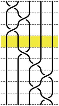
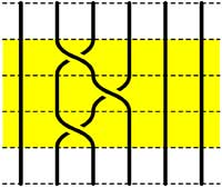
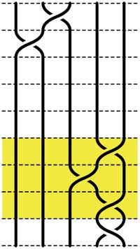
n-braids can be multiplied by putting them on top of each other and connecting the outputs of the first braid trivially to the inputs of the second. For example the 5-braid on the left can be written as $B=B_1.B_2 $ with $B_1 $ the braid on the top 3 subintervals and $B_2 $ the braid on the lower 5 subintervals.
In this way (and using our claim that there can be at most 1 crossing in each subinterval) we can write any n-braid as a word in the generators $\sigma_i $ (with $1 \leq i < n $) being the overcrossing between inputs i and i+1. Observe that the undercrossing is then the inverse $\sigma_i^{-1} $. For example, the braid on the left corresponds to the word
$\sigma_1^{-1}.\sigma_2^{-1}.\sigma_1^{-1}.\sigma_2.\sigma_3^{-1}.\sigma_4^{-1}.\sigma_3^{-1}.\sigma_4 $
Clearly there are relations among words in the generators. The easiest one we have already used implicitly namely that $\sigma_i.\sigma_i^{-1} $ is the trivial braid. Emil Artin proved in the 1930-ies that all such relations are consequences of two sets of ‘obvious’ relations. The first being commutation relations between crossings when the strings are far enough from each other. That is we have
$\sigma_i . \sigma_j = \sigma_j . \sigma_i $ whenever $|i-j| \geq 2 $
 =
= 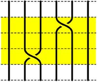
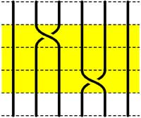
The second basic set of relations involves crossings using a common string
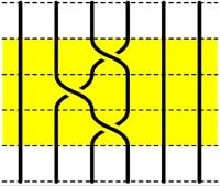
$\sigma_i.\sigma_{i+1}.\sigma_i = \sigma_{i+1}.\sigma_i.\sigma_{i+1} $
 =
=
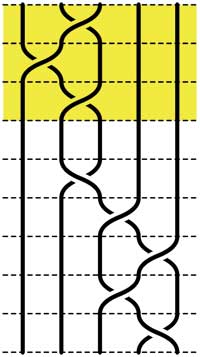
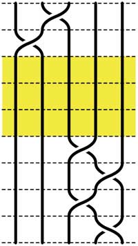
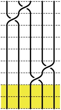
Starting with the 5-braid at the top, we can use these relations to reduce it to a simpler form. At each step we have outlined to region where the relations are applied
 =
= =
= =
=
These beautiful braid-pictures were produced using the braid-metapost program written by Stijn Symens.
Tracing a string from an input to an output assigns to an n-braid a permutation on n letters. In the above example, the permutation is $~(1,2,4,5,3) $. As this permutation doesn’t change under applying basic reduction, this gives a group-morphism
$\mathbb{B}_n \rightarrow S_n $
from the braid group on n strings $\mathbb{B}_n $ to the symmetric group. We have seen before that the symmetric group $S_n $ has a F-un interpretation as the linear group $GL_n(\mathbb{F}_1) $ over the field with one element. Hence, we can ask whether there is also a F-un interpretation of the n-string braid group and of the above group-morphism.
Kapranov and Smirnov suggest in their paper that the n-string braid group $\mathbb{B}_n \simeq GL_n(\mathbb{F}_1[t]) $ is the general linear group over the polynomial ring $\mathbb{F}_1[t] $ over the field with one element and that the evaluation morphism (setting t=0)
$GL_n(\mathbb{F}_1[t]) \rightarrow GL_n(\mathbb{F}1) $ gives the groupmorphism $\mathbb{B}_n \rightarrow S_n $
The rationale behind this analogy is a theorem of Drinfeld‘s saying that over a finite field $\mathbb{F}_q $, the profinite completion of $GL_n(\mathbb{F}_q[t]) $ is embedded in the fundamental group of the space of q-polynomials of degree n in much the same way as the n-string braid group $\mathbb{B}_n $ is the fundamental group of the space of complex polynomials of degree n without multiple roots.
And, now that we know the basics of absolute linear algebra, we can give an absolute braid-group representation
$\mathbb{B}_n = GL_n(\mathbb{F}_1[t]) \rightarrow GL_n(\mathbb{F}_{1^n}) $
obtained by sending each generator $\sigma_i $ to the matrix over $\mathbb{F}_{1^n} $ (remember that $\mathbb{F}_{1^n} = (\mu_n)^{\bullet} $ where $\mu_n = \langle \epsilon_n \rangle $ are the n-th roots of unity)
$\sigma_i \mapsto \begin{bmatrix}
1_{i-1} & & & \\
& 0 & \epsilon_n & \\
& \epsilon_n^{-1} & 0 & \\
& & & 1_{n-1-i} \end{bmatrix} $
and it is easy to see that these matrices do indeed satisfy Artin’s defining relations for $\mathbb{B}_n $.
5 Comments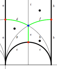
 We have
  On the left, a quilt-diagram copied from Hsu’s book