neverendingbooks

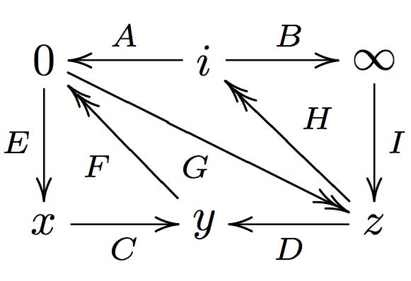
We have associated to a subgroup of the modular group $PSL_2(\mathbb{Z}) $ a quiver (that is, an oriented graph). For example, one verifies that the fundamental domain of the subgroup $\Gamma_0(2) $ (an index 3 subgroup) is depicted on the right by the region between the thick lines with the identification of edges as indicated. The associated quiver is then

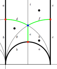
The corresponding “dessin d’enfant” are the green edges in the picture. But, the red dot on the left boundary is identied with the red dot on the lower circular boundary, so the dessin of the modular subgroup $\Gamma_0(2) $ is

Here, the three red dots (all of them even points in the Dedekind tessellation) give (after the identification) the two points indicated by a $\mid $ whereas the blue dot (an odd point in the tessellation) is depicted by a $\bullet $. There is another ‘quiver-like’ picture associated to this dessin, a quilt of the modular subgroup $\Gamma_0(2) $ as studied by John Conway and Tim Hsu.

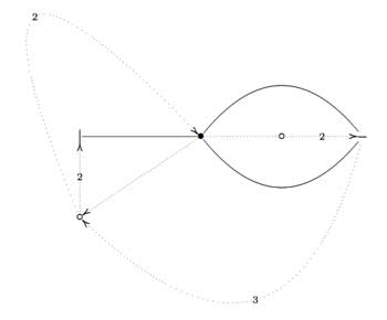
On the left, a quilt-diagram copied from Hsu’s book Quilts : central extensions, braid actions, and finite groups, exercise 3.3.9. This ‘quiver’ has also 5 vertices and 7 arrows as our quiver above, so is there a connection?

A quilt is a gadget to study transitive permutation representations of the braid group $B_3 $ (rather than its quotient, the modular group $PSL_2(\mathbb{Z}) = B_3/\langle Z \rangle $ where $\langle Z \rangle $ is the cyclic center of $B_3 $. The $Z $-stabilizer subgroup of all elements in a transitive permutation representation of $B_3 $ is the same and hence of the form $\langle Z^M \rangle $ where M is called the modulus of the representation. The arrow-data of a quilt, that is the direction of certain edges and their labeling with numbers from $\mathbb{Z}/M \mathbb{Z} $ (which have to satisfy some requirements, the flow rules, but more about that another time) encode the Z-action on the permutation representation. The dimension of the representation is $M \times k $ where $k $ is the number of half-edges in the dessin. In the above example, the modulus is 5 and the dessin has 3 (half)edges, so it depicts a 15-dimensional permutation representation of $B_3 $.

If we forget the Z-action (that is, the arrow information), we get a permutation representation of the modular group (that is a dessin). So, if we delete the labels and directions on the edges we get what Hsu calls a modular quilt, that is, a picture consisting of thick edges (the dessin) together with dotted edges which are called the seams of the modular quilt. The modular quilt is merely another way to depict a fundamental domain of the corresponding subgroup of the modular group. For the above example, we have the indicated correspondences between the fundamental domain of $\Gamma_0(2) $ in the upper half-plane (on the left) and as a modular quilt (on the right)

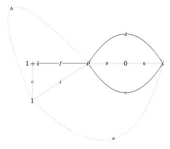
That is, we can also get our quiver (or its opposite quiver) from the modular quilt by fixing the orientation of one 2-cell. For example, if we fix the orientation of the 2-cell $\vec{fch} $ we get our quiver back from the modular quilt

This shows that the quiver (or its opposite) associated to a (conjugacy class of a) subgroup of $PSL_2(\mathbb{Z}) $ does not depend on the choice of embedding of the dessin (or associated cuboid tree diagram) in the upper half-plane. For, one can get the modular quilt from the dessin by adding one extra vertex for every connected component of the complement of the dessin (in the example, the two vertices corresponding to 0 and 1) and drawing a triangulation from them (the dotted lines or ‘seams’).

Last time we have that that one can represent (the conjugacy class of) a finite index subgroup of the modular group $\Gamma = PSL_2(\mathbb{Z}) $ by a Farey symbol or by a dessin or by its fundamental domain. Today we will associate a quiver to it.

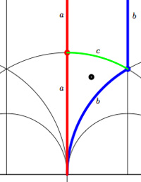
For example, the modular group itself is represented by the Farey symbol
or by its dessin (the green circle-edge) or by its fundamental domain which is the region of the upper halfplane bounded by the red and blue vertical boundaries. Both the red and blue boundary consist of TWO edges which are identified with each other and are therefore called a and b. These edges carry a natural orientation given by circling counter-clockwise along the boundary of the marked triangle (or clockwise along the boundary of the upper unmarked triangle having $\infty $ as its third vertex). That is the edge a is oriented from $i $ to $0 $ (or from $i $ to $\infty $) and the edge b is oriented from $0 $ to $\rho $ (or from $\infty $ to $\rho $) and the green edge c (which is an inner edge so carries no identifications) from $\rho $ to $i $. That is, the fundamental region consists of two triangles, glued together along their boundary which is the oriented cycle $\vec{abc} $ consistent with the fact that the compactification of $\mathcal{H}/\Gamma $ is the 2-sphere $S^2 = \mathbb{P}^1_{\mathbb{C}} $. Under this identification the triangle-boundary abc can be seen to circle the equator whereas the top triangle gives the upper half sphere and the lower triangle the lower half sphere. Emphasizing the orientation we can depict the triangle-boundary as the quiver

embedded in the 2-sphere. Note that quiver is just a fancy name for an oriented graph…

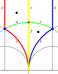
Okay, let’s look at the next case, that of the unique index 2 subgroup $\Gamma_2 $ represented by the Farey symbol or the dessin (the two green edges) or by its fundamental domain consisting of the 4 triangles where again the left and right vertical boundaries are to be identified in parts.

That is we have 6 edges on the 2-sphere $\mathcal{H}/\Gamma_2 = S^2 $ all of them oriented by the above rule. So, for example the lower-right triangle is oriented as $\vec{cfb} $. To see how this oriented graph (the quiver) is embedded in $S^2 $ view the big lower region (cdab) as the under hemisphere and the big upper region (abcd) as the upper hemisphere. So, the two green edges together with a and b are the equator and the remaining two yellow edges form the two parts of a bigcircle connecting the north and south pole. That is, the graph are the cut-lines if we cut the sphere in 4 equal parts. The corresponding quiver-picture is

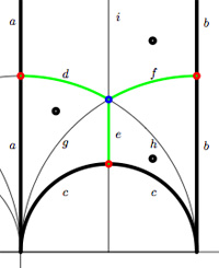
As a mental check, verify that the index 3 subgroup determined by the Farey symbol , whose fundamental domain with identifications is given on the left, has as its associated quiver picture

whereas the index 3 subgroup determined by the Farey symbol , whose fundamental domain with identifications is depicted on the right, has as its associated quiver

Next time, we will use these quivers to define superpotentials…

Yesterday, Jan Stienstra gave a talk at theARTS entitled “Quivers, superpotentials and Dimer Models”. He started off by telling that the talk was based on a paper he put on the arXiv Hypergeometric Systems in two Variables, Quivers, Dimers and Dessins d’Enfants but that he was not going to say a thing about dessins but would rather focuss on the connection with superpotentials instead…pleasing some members of the public, while driving others to utter despair.

Anyway, it gave me the opportunity to figure out for myself what dessins might have to do with dimers, whathever these beasts are. Soon enough he put on a slide containing the definition of a dimer and from that moment on I was lost in my own thoughts… realizing that a dessin d’enfant had to be a dimer for the Dedekind tessellation of its associated Riemann surface!
and a few minutes later I could slap myself on the head for not having thought of this before :

There is a natural way to associate to a Farey symbol (aka a permutation representation of the modular group) a quiver and a superpotential (aka a necklace) defining (conjecturally) a Calabi-Yau algebra! Moreover, different embeddings of the cuboid tree diagrams in the hyperbolic plane may (again conjecturally) give rise to all sorts of arty-farty fanshi-wanshi dualities…

I’ll give here the details of the simplest example I worked out during the talk and will come back to general procedure later, when I’ve done a reference check. I don’t claim any originality here and probably all of this is contained in Stienstra’s paper or in some physics-paper, so if you know of a reference, please leave a comment. Okay, remember the Dedekind tessellation ?

So, all hyperbolic triangles we will encounter below are colored black or white. Now, take a Farey symbol and consider its associated special polygon in the hyperbolic plane. If we start with the Farey symbol

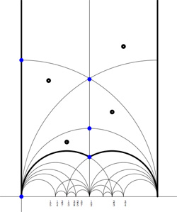
we get the special polygonal region bounded by the thick edges, the vertical edges are identified as are the two bottom edges. Hence, this fundamental domain has 6 vertices (the 5 blue dots and the point at $i \infty $) and 8 hyperbolic triangles (4 colored black, indicated by a black dot, and 4 white ones).

Right, now let us associate a quiver to this triangulation (which embeds the quiver in the corresponding Riemann surface). The vertices of the triangulation are also the vertices of the quiver (so in our case we are going for a quiver with 6 vertices). Every hyperbolic edge in the triangulation gives one arrow in the quiver between the corresponding vertices. The orientation of the arrow is determined by the color of a triangle of which it is an edge : if the triangle is black, we run around its edges counter-clockwise and if the triangle is white we run over its edges clockwise (that is, the orientation of the arrow is independent of the choice of triangles to determine it). In our example, there is one arrows directed from the vertex at $i $ to the vertex at $0 $, whether you use the black triangle on the left to determine the orientation or the white triangle on the right. If we do this for all edges in the triangulation we arrive at the quiver below

where x,y and z are the three finite vertices on the $\frac{1}{2} $-axis from bottom to top and where I’ve used the physics-convention for double arrows, that is there are two F-arrows, two G-arrows and two H-arrows. Observe that the quiver is of Calabi-Yau type meaning that there are as much arrows coming into a vertex as there are arrows leaving the vertex.

Now that we have our quiver we determine the superpotential as follows. Fix an orientation on the Riemann surface (for example counter-clockwise) and sum over all black triangles the product of the edge-arrows counterclockwise MINUS sum over all white triangles
the product of the edge arrows counterclockwise. So, in our example we have the cubic superpotential

$IH’B+HAG+G’DF+FEC-BHI-H’G'A-GFD-CEF’ $

From this we get the associated noncommutative algebra, which is the quotient of the path algebra of the above quiver modulo the following ‘commutativity relations’

$\begin{cases} GH &=G’H’ \\ IH’ &= IH \\ FE &= F’E \\ F’G’ &= FG \\ CF &= CF’ \\ EC &= GD \\ G’D &= EC \\ HA &= DF \\ DF’ &= H’A \\ AG &= BI \\ BI &= AG’ \end{cases} $

and morally this should be a Calabi-Yau algebra¹. This concludes the walk through of the procedure. Summarizing : to every Farey-symbol one associates a Calabi-Yau quiver and superpotential, possibly giving a Calabi-Yau algebra!

1. can someone who knows more about CYs verify this? [↩]

Warning: copy(62b064e4c60baad1e482ed4fcf366116.gif) [function.copy]: failed to open stream: No such file or directory in /Library/WebServer/Documents/latexrender/class.latexrender.php on line 321

Warning: unlink(/Library/WebServer/Documents/latexrender/tmp/62b064e4c60baad1e482ed4fcf366116.dvi) [function.unlink]: No such file or directory in /Library/WebServer/Documents/latexrender/class.latexrender.php on line 341

Warning: unlink(/Library/WebServer/Documents/latexrender/tmp/62b064e4c60baad1e482ed4fcf366116.ps) [function.unlink]: No such file or directory in /Library/WebServer/Documents/latexrender/class.latexrender.php on line 342

Warning: unlink(/Library/WebServer/Documents/latexrender/tmp/62b064e4c60baad1e482ed4fcf366116.gif) [function.unlink]: No such file or directory in /Library/WebServer/Documents/latexrender/class.latexrender.php on line 343

Take an affine $\mathbb{C} $-algebra A (not necessarily commutative). We will assign to it a strange object called the tangent-quiver $\vec{t}~A $, compute it in a few examples and later show how it connects with existing theory and how it can be used. This series of posts can be seen as the promised notes of my talks at the GAMAP-workshop but in reverse order… If some of the LaTeX-pictures are not in the desired spots, please size and resize your browser-window and they will find their intended positions.

A vertex $v $ of $\vec{t}~A $ corresponds to the isomorphism class of a finite dimensional simple A-representations $S_v $ and between any two such vertices, say $v $ and $w $, the number of directed arrows from $v $ to $w $ is given by the dimension of the Ext-space

$dim_{\mathbb{C}}~Ext^1_A(S_v,S_w) $

Recall that this Ext-space counts the equivalence classes of short exact sequences of A-representations

where two such sequences (say with middle terms V resp. W) are equivalent if there is an A-isomorphism $V \rightarrow^{\phi} W $ making the diagram below commutative

[Unparseable or potentially dangerous latex formula. Error 6 ]

The Ext-space measures how many non-split extensions there are between the two simples and is always a finite dimensional vectorspace. So the tangent quiver $\vec{t}~A $ has the property that in all vertices there are at most finitely many loops and between any two vertices there are a finite number of directed arrows, but in principle a vertex may be the origin of arrows connecting it to infinitely many other vertices.

Right, now let us at least motivate the terminology. Let $X $ be a (commutative) affine variety with coordinate ring $A = \mathbb{C}[X] $ then what is $\vec{t}~A $ in this case? To begin, as $\mathbb{C}[X] $ is commutative, all its finite dimensional simple representations are one-dimensional and there is one such for every point $x \in X $. Therefore, the vertices of $\vec{t}~A $ correspond to the points of the affine variety $X $. The simple A-representation $S_x $ corresponding to a point $x $ is just evaluating polynomials in $x $. Moreover, if $x \not= y $ then there are no non-split extensions between $S_x $ and $S_y $ (a commutative semi-local algebra splits as a direct sum of locals), therefore in $\vec{t}~A $ there can only be loops and no genuine arrows between different vertices. Finally, the number of loops in the vertex corresponding to the point $x $ can be computed using the fact that the self-extensions can be identified with the tangent space at $x $, that is

$dim_{\mathbb{C}}~Ext^1_{\mathbb{C}[X]}(S_x,S_x) = dim_{\mathbb{C}}~T_x~X $

That is, if $A=\mathbb{C}[X] $ is the coordinate ring of an affine variety $X $, then the quiver $\vec{t}~A $ is the set of points of $X $ having in each point $x $ as many loops as the dimension of the tangent space $T_x~X $. So, in this case, the quiver $\vec{t}~A $ contains all information about tangent spaces to the variety and that’s why we call it the tangent quiver.

Let’s go into the noncommutative wilderness. A first, quite trivial, example is the group algebra $A = \mathbb{C} G $ of a finite group $G $, then the simple A-representations are just the irreducible G-representations and as the group algebra is semi-simple every short exact sequence splits so all Ext-spaces are zero. That is, in this case the tangent quiver $\vec{t}~A $ in just a finite set of vertices (as many as there are irreducible G-representations) and no arrows nor loops.

Now you may ask whether there are examples of tangent quivers having arrows apart from loops. So, take another easy finite dimensional example : the path algebra $A = \mathbb{C} Q $ of a finite quiver $Q $ without oriented cycles. Recall that the path algebra is the vectorspace having as basis all vertices and all oriented paths in the quiver Q (and as there are no cycles, this basis is finite) and multiplication is induced by concatenation of paths. Here an easy example. Suppose the quiver Q looks like

then the path algebra is 6 dimensional as there are 3 vertices, 2 paths of length one (the arrows) and one path of length two (going from the leftmost to the rightmost vertex). The concatenation rule shows that the three vertices will give three idempotents in A and one easily verifies that the path algebra can be identified with upper-triangular $3 \times 3 $ matrices

$\mathbb{C} Q \simeq \begin{bmatrix} \mathbb{C} & \mathbb{C} & \mathbb{C} \\\ 0 & \mathbb{C} & \mathbb{C} \\\ 0 & 0 & \mathbb{C} \end{bmatrix} $

where the diagonal components correspond to the vertices, the first offdiagonal components to the two arrows and the corner component corresponds to the unique path of length two. Right, for a general finite quiver without oriented cycles is the quite easy to see that all finite dimensional simples are one-dimensional and correspond to the vertex-idempotents, that is every simple is of the form $S_v = e_v \mathbb{C} Q e_v $ where $e_v $ is the vertex idempotent. No doubt, you can guess what the tangent quiver $\vec{t}~A = \vec{t}~\mathbb{C} Q $ will be, can’t you?

The categorical cafe has a guest post by Tom Leinster Linear Algebra Done Right on the book with the same title by Sheldon Axler. I haven’t read the book but glanced through his online paper Down with determinants!. Here is ‘his’ proof of the fact that any n by n matrix A has at least one eigenvector. Take a vector $v \in \mathbb{C}^n $, then as the collection of vectors ${ v,A.v,A^2.v,\ldots,A^n.v } $ must be linearly dependent, there are complex numbers $a_i \in \mathbb{C} $ such that $~(a_0 + a_1 A + a_2 A^2 + \ldots + a_n A^n).v = \vec{0} \in \mathbb{C}^n $ But then as $\mathbb{C} $ is algebraically closed the polynomial on the left factors into linear factors $a_0 + a_1 x + a_2 x^2 + \ldots + a_n x^n = c (x-r_1)(x-r_2) \ldots (x-r_n) $ and therefore as $c(A-r_1I_n)(A-r_2I_n) \ldots (A-r_nI_n).v = \vec{0} $ from which it follows that at least one of the linear transformations $A-r_j I_n $ has a non-trivial kernel, whence A has an eigenvector with eigenvalue $r_j $. Okay, fine, nice even, but does this simple minded observation warrant the extreme conclusion of his paper (on page 18) ?

As mathematicians, we often read a nice new proof of a known theorem, enjoy the different approach, but continue to derive our internal understanding from the method we originally learned. This paper aims to change drastically the way mathematicians think about and teach crucial aspects of linear algebra.

The simple proof of the existence of eigenvalues given in Theorem 2.1 should be the one imprinted in our minds, written on our blackboards, and published in our textbooks. Generalized eigenvectors should become a central tool for the understanding of linear operators. As we have seen, their use leads to natural definitions of multiplicity and the characteristic polynomial. Every mathematician and every linear algebra student should at least remember that the generalized eigenvectors of an operator always span the domain (Proposition 3.4)—this crucial result leads to easy proofs of upper-triangular form (Theorem 6.2) and the Spectral Theorem (Theorems 7.5 and 8.3).

Determinants appear in many proofs not discussed here. If you scrutinize such proofs, you’ll often discover better alternatives without determinants. Down with Determinants!

I welcome all new proofs of known results as they allow instructors to choose the one best suited to their students (and preferable giving more than one proof showing that there is no such thing as ‘the best way’ to prove a mathematical result). What worries me is Axler’s attitude shared by extremists and dogmatics world-wide : they are so blinded by their own right that they impoverish their own lifes (and if they had their way, also that of others) by not willing to consider other alternatives. A few other comments :

1. I would be far more impressed if he had given a short argument for the one line he skates over in his proof, that of $\mathbb{C} $ being algebraically closed. Does anyone give a proof of this fact anymore or is this one of the few facts we expect first year students to accept on faith?

   1. I dont understand this aversity to the determinant (probably because of its nonlinear character) but at the same time not having any problems with successive powers of matrices. Surely he knows that the determinant is a fixed $~\mathbb{Q}~ $-polynomial in the traces (which are linear!) of powers of the matrix.

   2. The essense of linear algebra is that by choosing a basis cleverly one can express a linear operator in a extremely nice matrix form (a canonical form) so that all computations become much more easy. This crucial idea of considering different bases and their basechange seems to be missing from Axler’s approach. Moreover, I would have thought that everyone would know these days that ‘linear algebra done right’ is a well developed topic called ‘representation theory of quivers’ but I realize this might be viewed as a dogmatic statement. Fortunately someone else is giving the basic linear algebra courses here in Antwerp so students are spared my private obsessions (at least the first few years…). In [his post](http://golem.ph.utexas.edu/category/2007/05/ linear_algebra_done_right.html) Leistner askes “What are determinants good for?” I cannot resist mentioning a trivial observation I made last week when thinking once again about THE rationality problem and which may be well known to others. Recall from the previous post that rationality of the quotient variety of matrix-couples $~(A,B) \in M_n(\mathbb{C}) \oplus M_n(\mathbb{C}) / GL_n $ under _simultaneous conjugation_ is a very hard problem. On the other hand, the ‘near miss’ problem of the quotient variety of matrix-couples $ { (A,B)~|~det(A)=0~} / GL_n $ is completely trivial. It is rational for all n. Here is a one-line proof. Consider the quiver $\xymatrix{\vtx{} \ar@/^2ex/[rr] & & \vtx{} \ar@(ur,dr) \ar@/^2ex/[ll]} $ then the dimension vector (n-1,n) is a Schur root and the first fundamental theorem of $GL_n $ (see for example Hanspeter Krafts excellent book on invariant theory) asserts that the corresponding quotient variety is the one above. The result then follows from Aidan Schofield’s paper Birational classification of moduli spaces of representations of quivers. Btw. in this special case one does not have to use the full force of Aidan’s result. Zinovy Reichstein, who keeps me updated on events in Atlanta, emailed the following elegant short proof Here is an outline of a geometric proof. Let $X = {(A, B) : det(A) = 0} \subset M_n^2 $ and $Y = \mathbb{P}^{n-1} \times M_n $. Applying the no-name lemma to the $PGL_n $-equivariant dominant rational map $~X \rightarrow Y $ given by $~(A, B) \rightarrow (Ker(A), B) $ (which makes X into a vector bundle over a dense open $PGL_n $-invariant subset of Y), we see that $X//PGL_n $ is rational over $Y//PGL_n $ On the other hand, $Y//PGLn = M_n//PGL_n $ is an affine space. Thus $X//PGL_n $ is rational. The moment I read this I knew how to do this quiver-wise and that it is just another Brauer-Severi type argument so completely inadequate to help settling the genuine matrix-problem. Update on the paper by Esther Beneish : Esther did submit the paper in february.