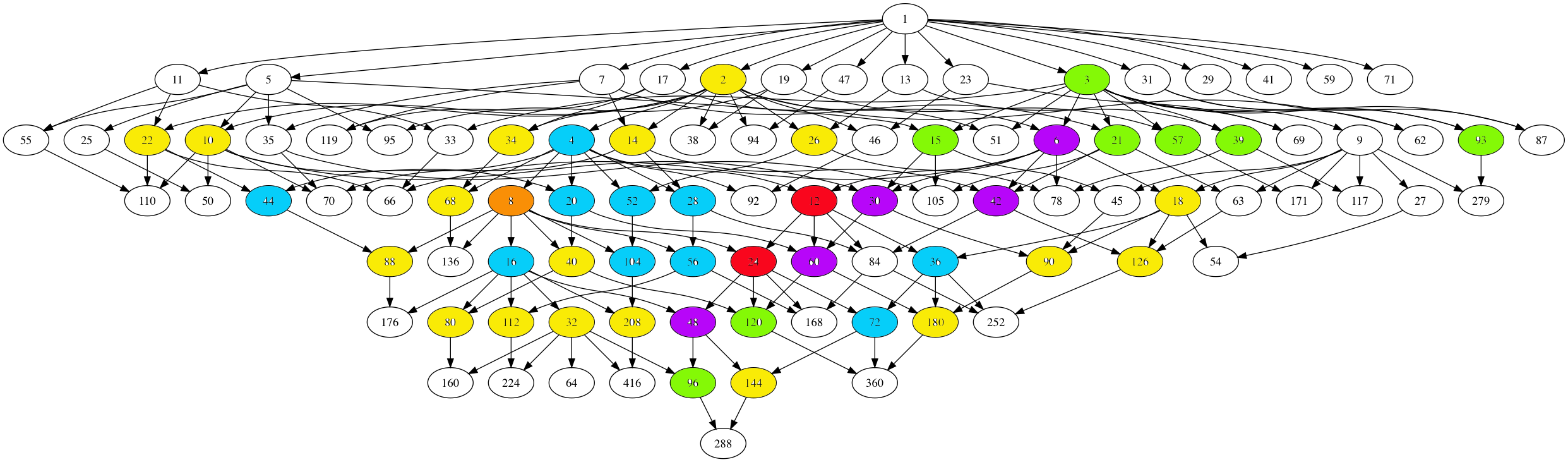
The monstrous moonshine picture is the finite piece of Conway’s Big Picture needed to understand the 171 moonshine groups associated to conjugacy classes of the monster.
Last time I claimed that there were exactly 7 types of local behaviour, but I missed one. The forgotten type is centered at the number lattice $84$.
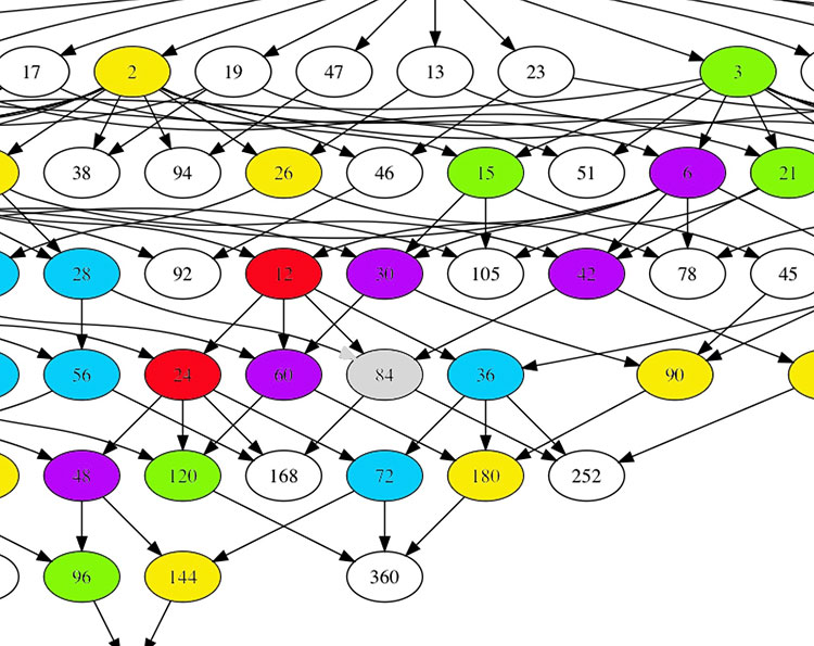
Locally around it the moonshine picture looks like this
\[
\xymatrix{42 \ar@{-}[dr] & 28 \frac{1}{3} \ar@[red]@{-}[d] & 41 \frac{1}{2} \ar@{-}[ld] \\ 28 \ar@[red]@{-}[r] & \color{grey}{84} \ar@[red]@{-}[r] \ar@[red]@{-}[d] \ar@{-}[rd] & 28 \frac{2}{3} \\ & 252 & 168} \]
and it involves all square roots of unity ($42$, $42 \frac{1}{2}$ and $168$) and $3$-rd roots of unity ($28$, $28 \frac{1}{3}$, $28 \frac{2}{3}$ and $252$) centered at $84$.
No, I’m not hallucinating, there are indeed $3$ square roots of unity and $4$ third roots of unity as they come in two families, depending on which of the two canonical forms to express a lattice is chosen.
In the ‘normal’ expression $M \frac{g}{h}$ the two square roots are $42$ and $42 \frac{1}{2}$ and the three third roots are $28, 28 \frac{1}{3}$ and $28 \frac{2}{3}$. But in the ‘other’ expression
\[
M \frac{g}{h} = (\frac{g’}{h},\frac{1}{h^2M}) \]
(with $g.g’ \equiv 1~mod~h$) the families of $2$-nd and $3$-rd roots of unity are
\[
\{ 42 \frac{1}{2} = (\frac{1}{2},\frac{1}{168}), 168 = (0,\frac{1}{168}) \} \]
and
\[
\{ 28 \frac{1}{3} = (\frac{1}{3},\frac{1}{252}), 28 \frac{2}{3} = (\frac{2}{3},\frac{1}{252}), 252 = (0 , \frac{1}{252}) \} \]
As in the tetrahedral snake post, it is best to view the four $3$-rd roots of unity centered at $84$ as the vertices of a tetrahedron with center of gravity at $84$. Power maps in the first family correspond to rotations along the axis through $252$ and power maps in the second family are rotations along the axis through $28$.
In the ‘normal’ expression of lattices there’s then a total of 8 different local types, but two of them consist of just one number lattice: in $8$ the local picture contains all square, $4$-th and $8$-th roots of unity centered at $8$, and in $84$ the square and $3$-rd roots.
Perhaps surprisingly, if we redo everything in the ‘other’ expression (and use the other families of roots of unity), then the moonshine picture has only 7 types of local behaviour. The forgotten type $84$ appears to split into two occurrences of other types (one with only square roots of unity, and one with only $3$-rd roots).
I wonder what all this has to do with the action of the Bost-Connes algebra on the big picture or with Plazas’ approach to moonshine via non-commutative geometry.
Leave a Comment