Huawei, the Chinese telecom giant, appears to support (and divide) the French mathematical community.
I was surprised to see that Laurent Lafforgue’s affiliation recently changed from ‘IHES’ to ‘Huawei’, for example here as one of the organisers of the Lake Como conference on ‘Unifying themes in geometry’.
Judging from this short Huawei-clip (in French) he thoroughly enjoys his new position.
Huawei claims that ‘Three more winners of the highest mathematics award have now joined Huawei’:
– Maxim Kontsevich, (IHES) Fields medal 1998
– Pierre-Louis Lions (College de France) Fields medal 1994
– Alessio Figalli (ETH) Fields medal 2018
These news-stories seem to have been G-translated from the Chinese, resulting in misspellings and perhaps other inaccuracies. Maxim’s research field is described as ‘kink theory’ (LoL).
Apart from luring away Fields medallist, Huawei set up last year the brand new Huawei Lagrange Research Center in the posh 7th arrondissement de Paris. (This ‘Lagrange Center’ is different from the Lagrange Institute in Paris devoted to astronomy and physics.)
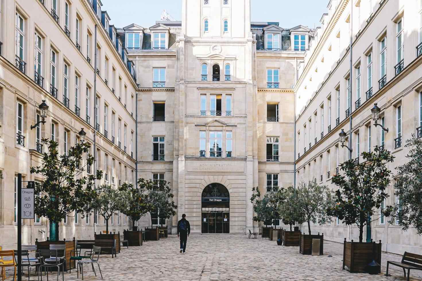
It aims to host about 30 researchers in mathematics and computer science, giving them the opportunity to live in the ‘unique eco-system of Paris, having the largest group of mathematicians in the world, as well as the best universities’.
Last May, Michel Broué authored an open letter to the French mathematical community Dans un hotel particulier du 7eme arrondissement de Paris (in French). A G-translation of the final part of this open letter:
“In the context of a very insufficient research and development effort in France, and bleak prospects for our young researchers, it is tempting to welcome the creation of the Lagrange center. We welcome the rise of Chinese mathematics to the highest level, and we are obviously in favour of scientific cooperation with our Chinese colleagues.
But in view of the role played by Huawei in the repression in Xinjiang and potentially everywhere in China, we call on mathematicians and computer scientists already engaged to withdraw from this project. We ask all researchers not to participate in the activities of this center, as we ourselves are committed to doing.”
Among the mathematicians signing the letter are Pierre Cartier and Pierre Schapira.
To be continued.
One Comment
 Of course, excellent math-blogs exist in every language imaginable, but my linguistic limitations restrict me to the ones written in English, French, German and … Dutch. Here a few links to Dutch (or rather, Flemish) math-blogs, in order of proximity :
 “This week I did spend much of my time at the Fifth European Mathematical Congress in Amsterdam. Several mathematicians suggested I should have a chat with