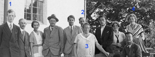
For the better part of the 30ties, Ernst Witt (1) did hang out with the rest of the ‘Noetherknaben’, the group of young mathematicians around Emmy Noether (3) in Gottingen.
In 1934 Witt became Helmut Hasse‘s assistent in Gottingen, where he qualified as a university lecturer in 1936. By 1938 he has made enough of a name for himself to be offered a lecturer position in Hamburg and soon became an associate professor, the down-graded position held by Emil Artin (2) until he was forced to emigrate in 1937.
A former fellow student of him in Gottingen, Erna Bannow (4), had gone earlier to Hamburg to work with Artin. She continued her studies with Witt and finished her Ph.D. in 1939. In 1940 Erna Bannow and Witt married.
So, life was smiling on Ernst Witt that sunday january 28th 1940, both professionally and personally. There was just one cloud on the horizon, and a rather menacing one. He was called up by the Wehrmacht and knew he had to enter service in february. For all he knew, he was spending the last week-end with his future wife… (later in february 1940, Blaschke helped him to defer his military service by one year).
Still, he desperately wanted to finish his paper before entering the army, so he spend most of that week-end going through the final version and submitted it on monday, as the published paper shows.
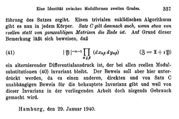
In the 70ties, Witt suddenly claimed he did discover the Leech lattice $ {\Lambda} $ that sunday. Last time we have seen that the only written evidence for Witt’s claim is one sentence in his 1941-paper Eine Identität zwischen Modulformen zweiten Grades. “Bei dem Versuch, eine Form aus einer solchen Klassen wirklich anzugeben, fand ich mehr als 10 verschiedene Klassen in $ {\Gamma_{24}} $.”
But then, why didn’t Witt include more details of this sensational lattice in his paper?
Ina Kersten recalls on page 328 of Witt’s collected papers : “In his colloquium talk “Gitter und Mathieu-Gruppen” in Hamburg on January 27, 1970, Witt said that in 1938, he had found nine lattices in $ {\Gamma_{24}} $ and that later on January 28, 1940, while studying the Steiner system $ {S(5,8,24)} $, he had found two additional lattices $ {M} $ and $ {\Lambda} $ in $ {\Gamma_{24}} $. He continued saying that he had then given up the tedious investigation of $ {\Gamma_{24}} $ because of the surprisingly low contribution
$ \displaystyle | Aut(\Lambda) |^{-1} < 10^{-18} $
to the Minkowski density and that he had consented himself with a short note on page 324 in his 1941 paper.”
In the last sentence he refers to the fact that the sum of the inverse orders of the automorphism groups of all even unimodular lattices of a given dimension is a fixed rational number, the Minkowski-Siegel mass constant. In dimension 24 this constant is
$ \displaystyle \sum_{L} \frac{1}{| Aut(L) |} = \frac {1027637932586061520960267}{129477933340026851560636148613120000000} \approx 7.937 \times 10^{-15} $
That is, Witt was disappointed by the low contribution of the Leech lattice to the total constant and concluded that there might be thousands of new even 24-dimensional unimodular lattices out there, and dropped the problem.
If true, the story gets even better : not only claims Witt to have found the lattices $ {A_1^{24}=M} $ and $ {\Lambda} $, but also enough information on the Leech lattice in order to compute the order of its automorphism group $ {Aut(\Lambda)} $, aka the Conway group $ {Co_0 = .0} $ the dotto-group!
Is this possible? Well fortunately, the difficulties one encounters when trying to compute the order of the automorphism group of the Leech lattice from scratch, is one of the better documented mathematical stories around.
The books From Error-Correcting Codes through Sphere Packings to Simple Groups by Thomas Thompson, Symmetry and the monster by Mark Ronan, and Finding moonshine by Marcus du Sautoy tell the story in minute detail.
It took John Conway 12 hours on a 1968 saturday in Cambridge to compute the order of the dotto group, using the knowledge of Leech and McKay on the properties of the Leech lattice and with considerable help offered by John Thompson via telephone.
But then, John Conway is one of the fastest mathematicians the world has known. The prologue of his book On numbers and games begins with : “Just over a quarter of a century ago, for seven consecutive days I sat down and typed from 8:30 am until midnight, with just an hour for lunch, and ever since have described this book as “having been written in a week”.”
Conway may have written a book in one week, Ernst Witt did complete his entire Ph.D. in just one week! In a letter of August 1933, his sister told her parents : “He did not have a thesis topic until July 1, and the thesis was to be submitted by July 7. He did not want to have a topic assigned to him, and when he finally had the idea, he started working day and night, and eventually managed to finish in time.”
So, if someone might have beaten John Conway in fast-computing the dottos order, it may very well have been Witt. Sadly enough, there is a lot of circumstantial evidence to make Witt’s claim highly unlikely.
For starters, psychology. Would you spend your last week-end together with your wife to be before going to war performing an horrendous calculation?
Secondly, mathematical breakthroughs often arise from newly found insight. At that time, Witt was also working on his paper on root lattices “Spiegelungsgrupen and Aufzähling halbeinfacher Liescher Ringe” which he eventually submitted in january 1941. Contained in that paper is what we know as Witt’s lemma which tells us that for any integral lattice the sublattice generated by vectors of norms 1 and 2 is a direct sum of root lattices.
This leads to the trick of trying to construct unimodular lattices by starting with a direct sum of root lattices and ‘adding glue’. Although this gluing-method was introduced by Kneser as late as 1967, Witt must have been aware of it as his 16-dimensional lattice $ {D_{16}^+} $ is constructed this way.
If Witt wanted to construct new 24-dimensional even unimodular lattices in 1940, it would be natural for him to start off with direct sums of root lattices and trying to add vectors to them until he got what he was after. Now, all of the Niemeier-lattices are constructed this way, except for the Leech lattice!
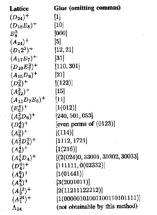
I’m far from an expert on the Niemeier lattices but I would say that Witt definitely knew of the existence of $ {D_{24}^+} $, $ {E_8^3} $ and $ {A_{24}^+} $ and that it is quite likely he also constructed $ {(D_{16}E_8)^+, (D_{12}^2)^+, (A_{12}^2)^+, (D_8^3)^+} $ and possibly $ {(A_{17}E_7)^+} $ and $ {(A_{15}D_9)^+} $. I’d rate it far more likely Witt constructed another two such lattices on sunday january 28th 1940, rather than discovering the Leech lattice.
Finally, wouldn’t it be natural for him to include a remark, in his 1941 paper on root lattices, that not every even unimodular lattices can be obtained from sums of root lattices by adding glue, the Leech lattice being the minimal counter-example?
If it is true he was playing around with the Steiner systems that sunday, it would still be a pretty good story he discovered the lattices $ {(A_2^{12})^+} $ and $ {(A_1^{24})^+} $, for this would mean he discovered the Golay codes in the process!
Which brings us to our next question : who discovered the Golay code?
 Mike Artin, David Mumford and