If machine learning, AI, and large language models are here to stay, there’s this inevitable conclusion:
Millennials are the last generation to grow up without tropical geometry
— Dave Jensen (@DaveJensenMath) April 6, 2023
At the start of this series, the hope was to find the topos of the unconscious. Pretty soon, attention turned to the shape of languages and LLMs.
In large language models all syntactic and semantic information is encoded is huge arrays of numbers and weights. It seems unlikely that $\mathbf{Set}$-valued presheaves will be useful in machine learning, but surely Huawei will prove me wrong.
$[0,\infty]$-enriched categories (aka generalised metric spaces) and associated $[0,\infty]$-enriched presheaves may be better suited to understand existing models.
But, as with ordinary presheaves, there are just too many $[0,\infty]$-enriched ones, So, how can we weed out the irrelevant ones?
For inspiration, let’s turn to evolutionary biology and their theory of phylogenetic trees. They want to trace back common (extinguished) ancestors of existing species by studying overlaps in the DNA.

(A tree of life, based on completely sequenced genomes, from Wikipedia)
The connection between phylogenetic trees and tropical geometry is nicely explained in the paper Tropical mathematics by David Speyer and Bernd Sturmfels.
The tropical semi-ring is the set $(-\infty,\infty]$, equipped with a new addition $\oplus$ and multiplication $\odot$
$$a \oplus b = min(a,b), \quad \text{and} \quad a \odot b = a+b$$
Because tropical multiplication is ordinary addition, a tropical monomial in $n$ variables
$$\underbrace{x_1 \odot \dots \odot x_1}_{j_1} \odot \underbrace{x_2 \odot \dots \odot x_2}_{j_2} \odot \dots$$
corresponds to the linear polynomial $j_1 x_1 + j_2 x_2 + \dots \in \mathbb{Z}[x_1,\dots,x_n]$. But then, a tropical polynomial in $n$ variables
$$p(x_1,\dots,x_n)=a \odot x_1^{i_1}\dots x_n^{i_n} \oplus b \odot x_1^{j_1} \dots x_n^{j_n} \oplus \dots$$
gives the piece-wise linear function on $p : \mathbb{R}^n \rightarrow \mathbb{R}$
$$p(x_1,\dots,x_n)=min(a+i_1 x_1 + \dots + i_n x_n,b+j_1 x_1 + \dots + j_n x_n, \dots)$$
The tropical hypersurface $\mathcal{H}(p)$ then consists of all points of $v \in \mathbb{R}^n$ where $p$ is not linear, that is, the value of $p(v)$ is attained in at least two linear terms in the description of $p$.
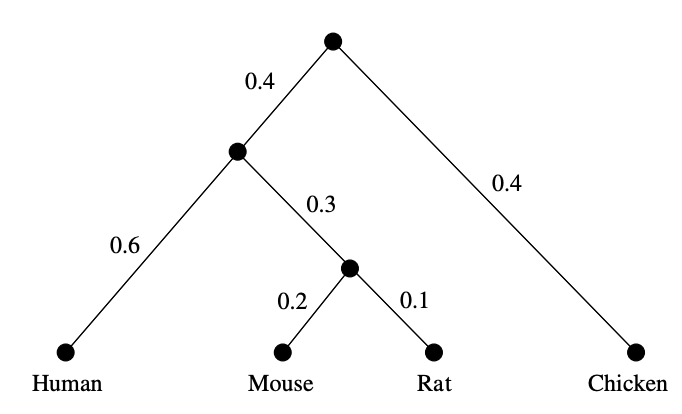
Now, for the relation to phylogenetic trees: let’s sequence the genomes of human, mouse, rat and chicken and compute the values of a suitable (necessarily symmetric) distance function between them:
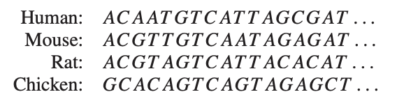
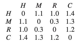
From these distances we want to trace back common ancestors and their difference in DNA-profile in a consistent manner, that is, such that the distance between two nodes in the tree is the sum of the distances of the edges connecting them.
In this example, such a tree is easily found (only the weights of the two edges leaving the root can be different, with sum $0.8$):
In general, let’s sequence the genomes of $n$ species and determine their distance matrix $D=(d_{ij})_{i,j}$. Biology asserts that this distance must be a tree-distance, and those can be characterised by the condition that for all $1 \leq i,j,k,l \leq n$, among the three numbers
$$d_{ij}+d_{kl},~d_{ik}+d_{jl},~d_{il}+d_{jk}$$
the maximum is attained at least twice.
What has this to do with tropical geometry? Well, $D$ is a tree distance if and only if $-D$ is a point in the tropical Grassmannian $Gr(2,n)$.
Here’s why: let $e_{ij}=-d_{ij}$ then the above condition is that the minimum of
$$e_{ij}+e_{kl},~e_{ik}+e_{jl},~e_{il}+e_{jk}$$
is attained at least twice, or that $(e_{ij})_{i,j}$ is a point of the tropical hypersurface
$$\mathcal{H}(x_{ij} \odot x_{kl} \oplus x_{ik} \odot x_{jl} \oplus x_{il} \odot x_{jk})$$
and we recognise this as one of the defining quadratic Plucker relations of the Grassmannian $Gr(2,n)$.
More on this can be found in another paper by Speyer and Sturmfels The tropical Grassmannian, and the paper Geometry of the space of phylogenetic trees by Louis Billera, Susan Holmes and Karen Vogtmann.
What’s the connection with $[0,\infty]$-enriched presheaves?
The set of all species $V=\{ m,n,\dots \}$ , together with the distance function $d(m,n)$ between their DNA-sequences is a $[0,\infty]$-category. Recall that a $[0,\infty]$-enriched presheaf on $V$ is a function $p : V \rightarrow [0,\infty]$ satisfying for all $m,n \in V$
$$d(m,n)+p(n) \geq p(m)$$
For an ancestor node $p$ we can take for every $m \in V$ as $p(m)$ the tree distance from $p$ to $m$, so every ancestor is a $[0,\infty]$-enriched presheaf.
We also defined the distance between such $[0,\infty]$-enriched presheaves $p$ and $q$ to be
$$\hat{d}(p,q) = sup_{m \in V}~max(q(m)-p(m),0)$$
and this distance coincides with the tree distance between the nodes.
So, all ancestors nodes in a phylogenetic tree are very special $[0,\infty]$-enriched presheaves, optimal for the connection with the underlying $[0,\infty]$-enriched category (the species and their differences in genome).
We would like to garden out such exceptional $[0,\infty]$-enriched presheaves in general, but clearly the underlying distance of a generalised metric space, even when it is symmetric, is not a tree metric.
Still, there might be regions in the space where we can do the above. So, in general we might expect not one tree, but a forest of trees formed by the $[0,\infty]$-enriched presheaves, optimal for the metric we’re exploring.
If we think of the underlying $[0,\infty]$-category as the conscious manifestations, then this forest of presheaves are the underlying brain-states (or, if you want, the unconscious) leading up to these.
That’s why I like to call this mental picture the tropical brain-forest.

(Image credit)
Where’s the tropical coming from?
Well, I think that in order to pinpoint these ‘optimal’ $[0,\infty]$-enriched presheaves a tropical-like structure on these, already mentioned by Simon Willerton in Tight spans, Isbell completions and semi-tropical modules, will be relevant.
For any two $[0,\infty]$-enriched presheaves we can take $p \oplus q = p \wedge q$, and for every $s \in [0,\infty]$ we can define
$$s \odot p : V \rightarrow [0,\infty] \qquad m \mapsto max(p(m)-s,0)$$
and check that this is again a $[0,\infty]$-presheaf. The mental idea of $s \odot p$ is that of a fat point centered at $p$ with size $s$.
(tbc)
Previously in this series:
- The topology of dreams
- The shape of languages
- Loading a second brain
- The enriched vault
- The super-vault of missing notes