“La Tribu” (“The Tribe”) was the internal Journal of the Bourbaki group between 1940 and 1977.
It’s main purpose was to record the editorial decisions made during the Bourbaki congresses, but it always started out with a humorous account of some of the events that happened during the meeting or in the world at large.
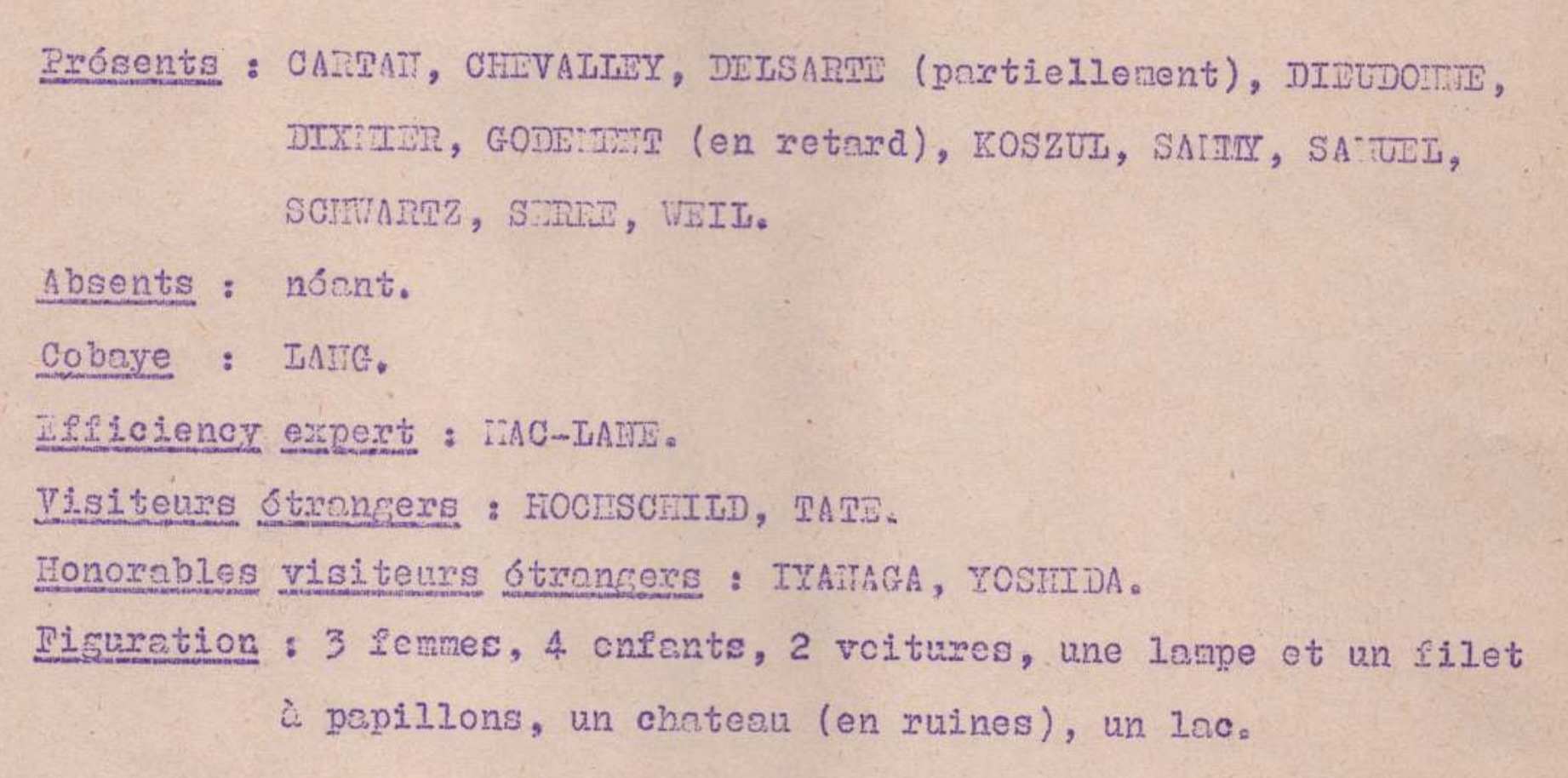
Every Tribe issue starts with a list of all people and things attending that meeting. Here’s one example, from the 1954 summer congress in Murols:
Some time ago, I’ve used the then available issues of “La Tribu” to locate the Hotels, Abbeys, Spas etc. where the Bourbaki congresses took place between 1940 and 1960. Here are some links:
In one of these post I pleaded:
“Dear Collaborators of Nicolas Bourbaki, please make all Bourbaki material (Diktat, La Tribu, versions) publicly available, certainly those documents older than 50 years.”
When I checked the Bourbaki Archives a few weeks ago, I was delighted to see that by now they have released all issues of “La Tribu” until 1973!
A few more places for me to locate, and a lot of fun intros to read.
From 1960 on, Cabris, in the Alpes-Maritime, near Grasse, and not too far from Cannes and Antibes, was by far the most popular congress spot for the second and third generation Bourbakistas.
Between 1960 and 1973 they visited the place no less than thirteen times, see the “La Tribu” issues nrs. 60,61,64,65,66,68,70,71,73,74,77,81 and 85.
Starting from 1965 they even held their annual two week summer conference there for five consecutive years.
Probably they kept returning there, even after 1973.
In the book Bourbaki, a secret society of mathematicians by Maurice Mashaal there are several photographs of the July 1975 Bourbaki Congress in Cabris.
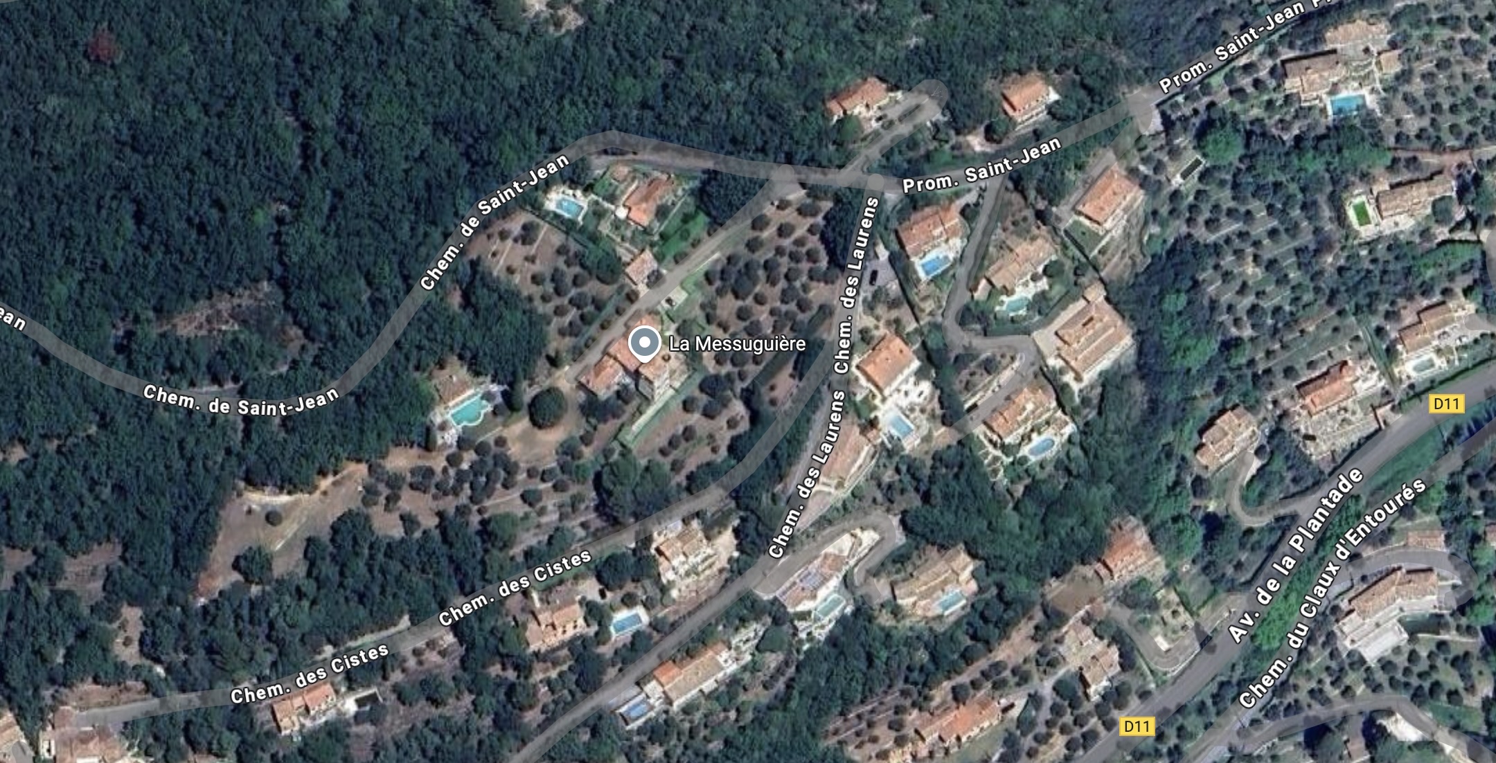
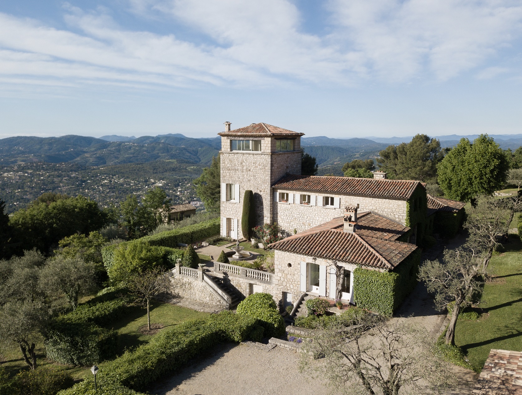
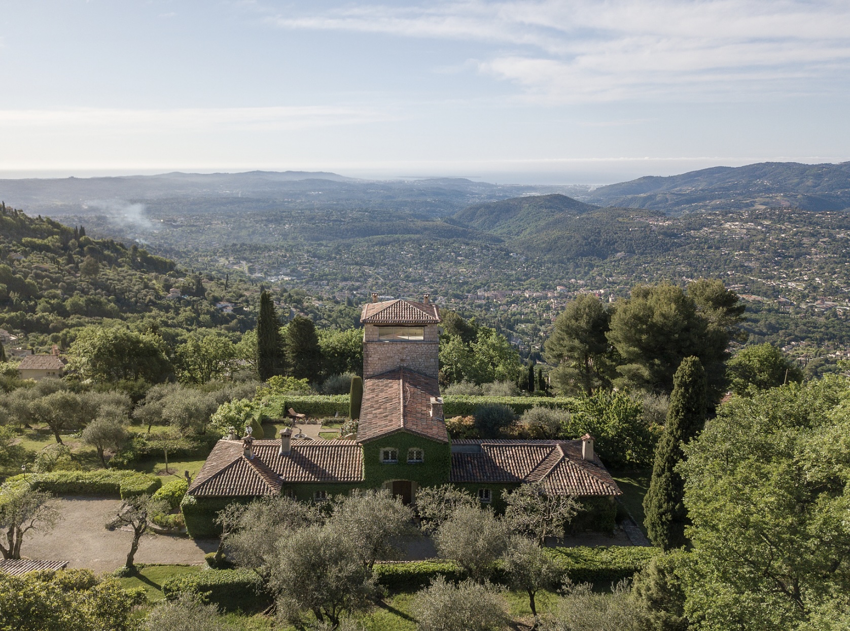
Finding their popular venue is quite easy, as “La Tribu” usually mentions “La Messuguiere, Cabris”.
(Photo credit)
The “Villa La Messuguiere” has an interesting history.
In 1938, Mrs. Mayrisch, formerly Aline de Saint-Hubert, purchased a plot of land in Cabris and built a house there, which she called La Messuguière. The name is derived from ‘le messugue’, the Provençal name for the cottony cistus, or Cistus albidus, a characteristic shrub of the ‘garrigue’ which thrives there.

She took refuge at La Messuguiere in 1940 and remained there until her death on January 20, 1947.
During the war, she welcomed her friends Andre Gide, Jean Schlumberger, Roger Martin
du Gard, Gaston Gallimard, Marie Delcourt, Alexis Curvers, Henri Michaux, and Andre Malraux.
Aline Mayrisch-de Saint-Hubert was attracted to the region because her friend Maria Van Rysselberghe, a Belgian writer and wife of the painter Theo Van Rysselberghe, lived at the ‘Villa Les Audides’, not far from La Messuguière.
Until 1979, Villa La Messuguiere hosted the French and international intellectual elite as paying guests. Gide was one of the first to settle there and received many visitors, among them: Henry de Montherlant, André Malraux and his wife Clara, Jean-Paul Sartre, and Albert Camus.
Clara Malraux wrote “Our Twenty Years” at the Villa, and Henri Thomas “The Promontory”, which earned him the Prix Fémina.
Apart from writers, also the philosopher Lucien Goldmann, the sociologist Georges Friedmann, the politician Jules Moch, and the micro-biologist and Nobel Prize winner Andre Lwoff stayed at La Messuguiere.
In the mid 1960s, at the height of their influence over French and international mathematics, the Bourbaki group probably only felt entitled to hold their meetings at this intellectual hotspot. Perhaps, the upcoming closure of the Villa as a conference centre in 1979 contributed to the rapid decline of the group in the late 1970s.
(Photo credit)