Category: groups

Here, MaMuTh stands for Mathematical Music Theory which analyses the pitch, timing, and structure of works of music.

The Elephant is the nickname for the ‘bible’ of topos theory, Sketches of an Elephant: A Topos Theory Compendium, a two (three?) volume book, written by Peter Johnstone.

How can we get as quickly as possible from the MaMuth to the Elephant, musical illiterates such as myself?

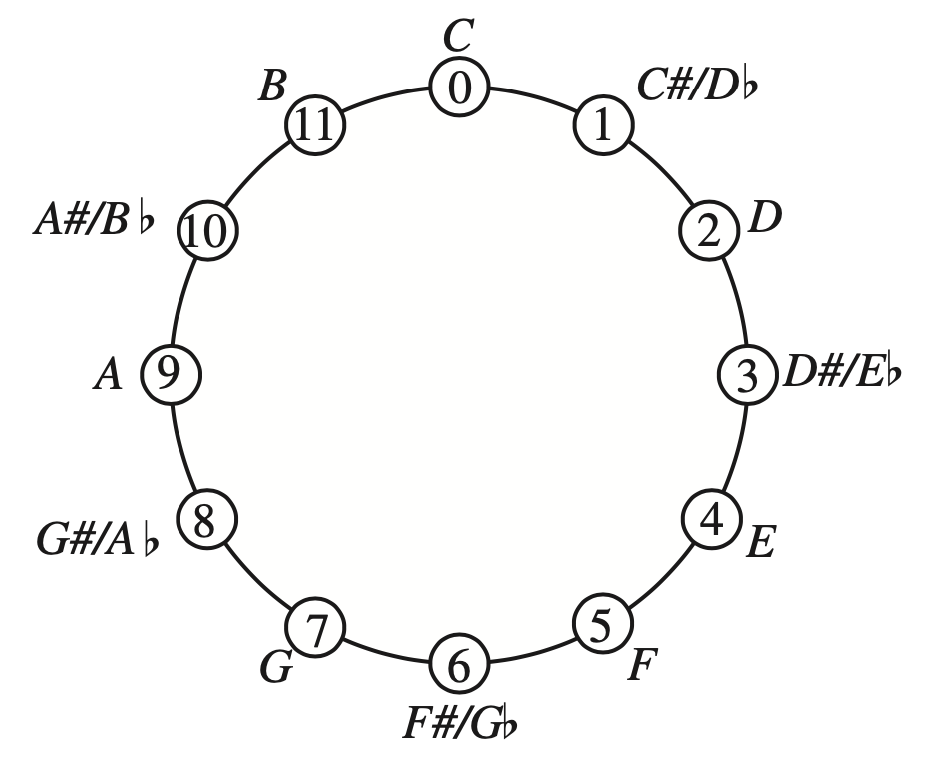
What Mamuth-ers call a pitch class (sounds that are a whole number of octaves apart), is for us a residue modulo $12$, as an octave is usually divided into twelve (half)tones.

We’ll just denote them by numbers from $0$ to $11$, or view them as the vertices of a regular $12$-gon, and forget the funny names given to them, as there are several such encodings, and we don’t know a $G$ from a $D\#$.

Our regular $12$-gon has exactly $24$ symmetries. Twelve rotations, which they call transpositions, given by the affine transformations
\[
T_k~:~x \mapsto x+k~\text{mod}~12 \]
and twelve reflexions, which they call involutions, given by
\[
I_k~:~x \mapsto -x+k~\text{mod}~12 \]
What for us is the dihedral group $D_{12}$ (all symmetries of the $12$-gon), is for them the $T/I$-group (for transpositions/involutions).

Let’s move from individual notes (or pitch classes) to chords (or triads), that is, three notes played together.

Not all triples of notes sound nice when played together, that’s why the most commonly played chords are among the major and minor triads.

A major triad is an ordered triple of elements from $\mathbb{Z}_{12}$ of the form
\[
(n,n+4~\text{mod}~12,n+7~\text{mod}~12) \]
and a minor triad is an ordered triple of the form
\[
(n,n+3~\text{mod}~12,n+7~\text{mod}~12) \]
where the first entry $n$ is called the root of the triad (or chord) and its funny name is then also the name of that chord.

For us, it is best to view a triad as an inscribed triangle in our regular $12$-gon. The triangles of major and minor triads have edges of different lengths, a small one, a middle, and a large one.

Starting from the root, and moving clockwise, we encounter in a major chord-triangle first the middle edge, then the small edge, and finally the large edge. For a minor chord-triangle, we have first the small edge, then the middle one, and finally the large edge.

On the left, two major triads, one with root $0$, the other with root $6$. On the right, two minor triads, also with roots $0$ and $6$.

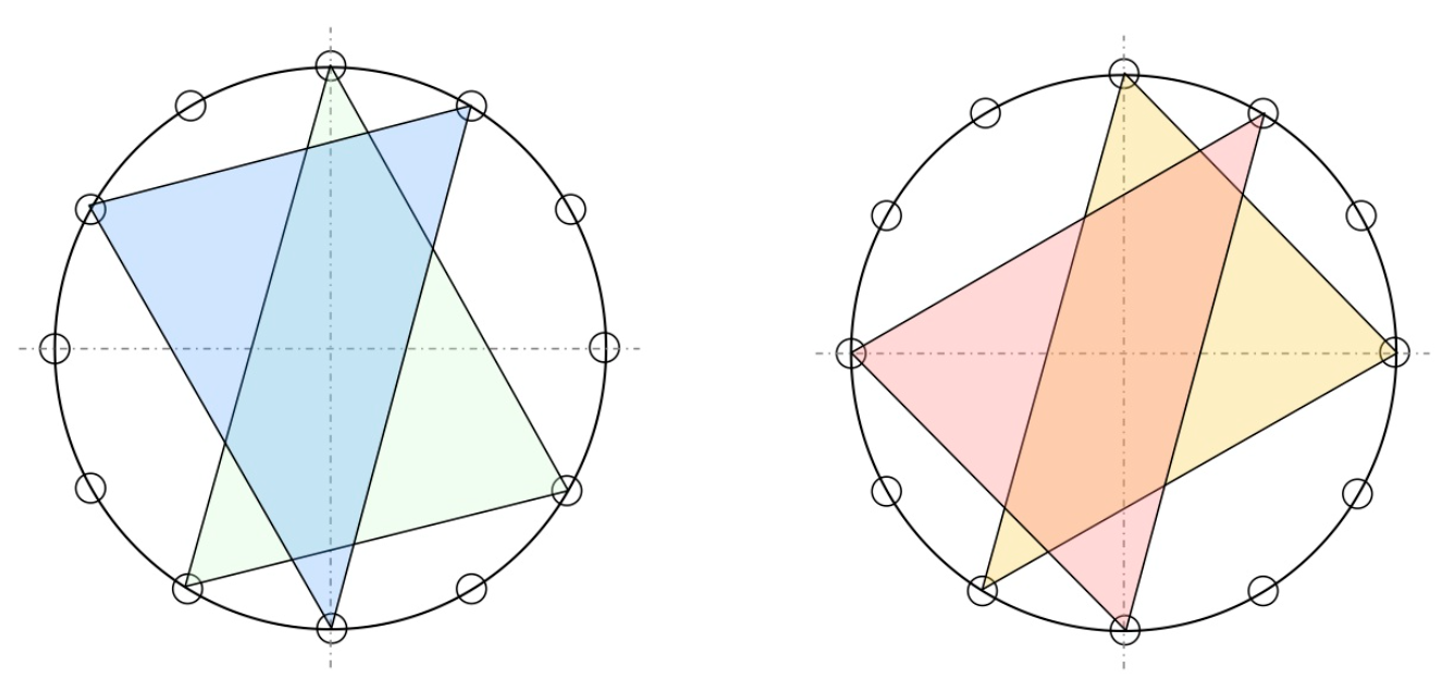
(Btw. if you are interested in the full musical story, I strongly recommend the alpof blog by Alexandre Popoff, from which the above picture is taken.)

Clearly, there are $12$ major triads (one for each root), and $12$ minor triads.

From the shape of the triad-triangles it is also clear that rotations (transpositions) send major triads to major triads (and minors to minors), and that reflexions (involutions) interchange major with minor triads.

That is, the dihedral group $D_{12}$ (or if you prefer the $T/I$-group) acts on the set of $24$ major and minor triads, and this action is transitive (an element stabilising a triad-triangle must preserve its type (so is a rotation) and its root (so must be the identity)).

Can we hear the action of the very special group element $T_6$ (the unique non-trivial central element of $D_{12}$) on the chords?

This action is not only the transposition by three full tones, but also a point-reflexion with respect to the center of the $12$-gon (see two examples in the picture above). This point reflexion can be compositionally meaningful to refer to two very different upside-down worlds.

In It’s $T_6$-day, Alexandre Popoff gives several examples. Here’s one of them, the Ark theme in Indiana Jones – Raiders of the Lost Ark.

“The $T_6$ transformation is heard throughout the map room scene (in particular at 2:47 in the video): that the ark is a dreadful object from a very different world is well rendered by the $T_6$ transposition, with its inherent tritone and point reflection.”

Let’s move on in the direction of the Elephant.

We saw that the only affine map of the form $x \mapsto \pm x + k$ fixing say the major $0$-triad $(0,4,7)$ is the identity map.

But, we can ask for the collection of all affine maps $x \mapsto a x + b$ fixing this major $0$-triad set-wise, that is, such that
\[
\{ b, 4a+b~\text{mod}~12, 7a+b~\text{mod}~2 \} \subseteq \{ 0,4,7 \} \]

A quick case-by-case analysis shows that there are just eight such maps: the identity and the constant maps
\[
x \mapsto x,~x \mapsto 0,~x \mapsto 4, ~x \mapsto 7 \]
and the four maps
\[
\underbrace{x \mapsto 3x+7}_a,~\underbrace{x \mapsto 8x+4}_b,~x \mapsto 9x+4,~x \mapsto 4x \]

Compositions of such maps again preserve the set $\{ 0,4,7 \}$ so they form a monoid, and a quick inspection with GAP learns that $a$ and $b$ generate this monoid.


gap> a:=Transformation([10,1,4,7,10,1,4,7,10,1,4,7]);;
gap> b:=Transformation([12,8,4,12,8,4,12,8,4,12,8,4]);;
gap> gens:=[a,b];;
gap> T:=Monoid(gens);
gap> Size(T);
8


The monoid $T$ is the triadic monoid of Thomas Noll’s paper The topos of triads.

The monoid $T$ can be seen as a one-object category (with endomorphisms the elements of $T$). The corresponding presheaf topos is then the category of all sets equipped with a right $T$-action.

Actually, Noll considers just one such presheaf (and its sub-presheaves) namely $\mathcal{F}=\mathbb{Z}_{12}$ with the action of $T$ by affine maps described before.

He is interested in the sheafifications of these presheaves with respect to Grothendieck topologies, so we have to describe those.

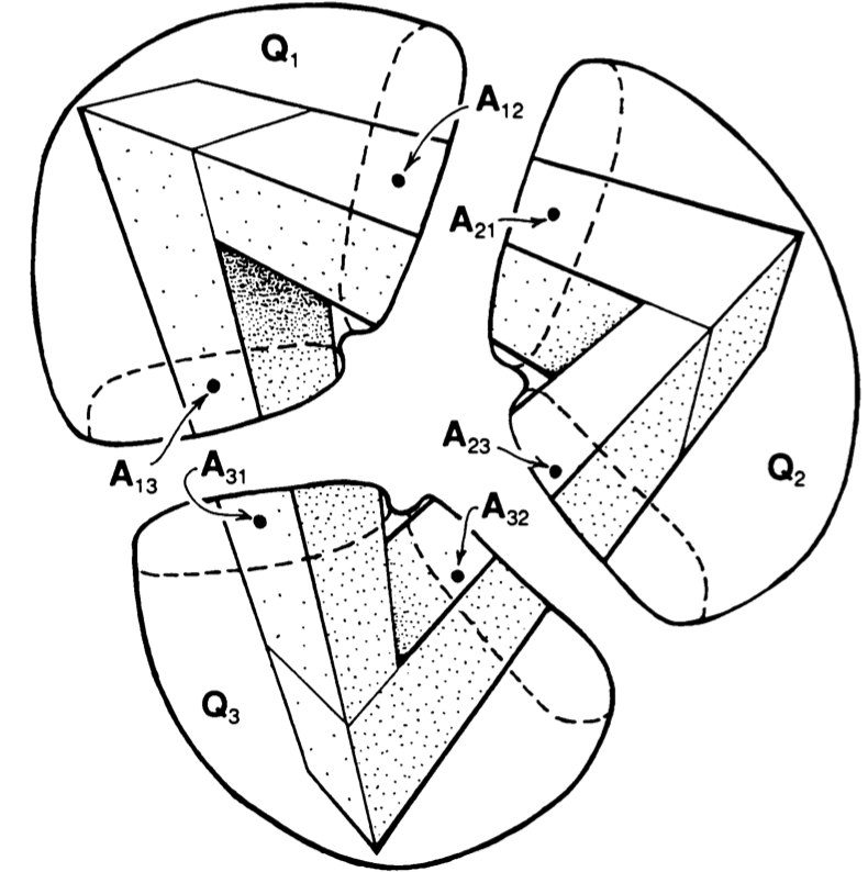
For any monoid category, the subobject classifier $\Omega$ is the set of all right ideals in the monoid.

Using the GAP sgpviz package we can draw its Cayley graph (red coloured vertices are idempotents in the monoid, the blue vertex is the identity map).


gap> DrawCayleyGraph(T);


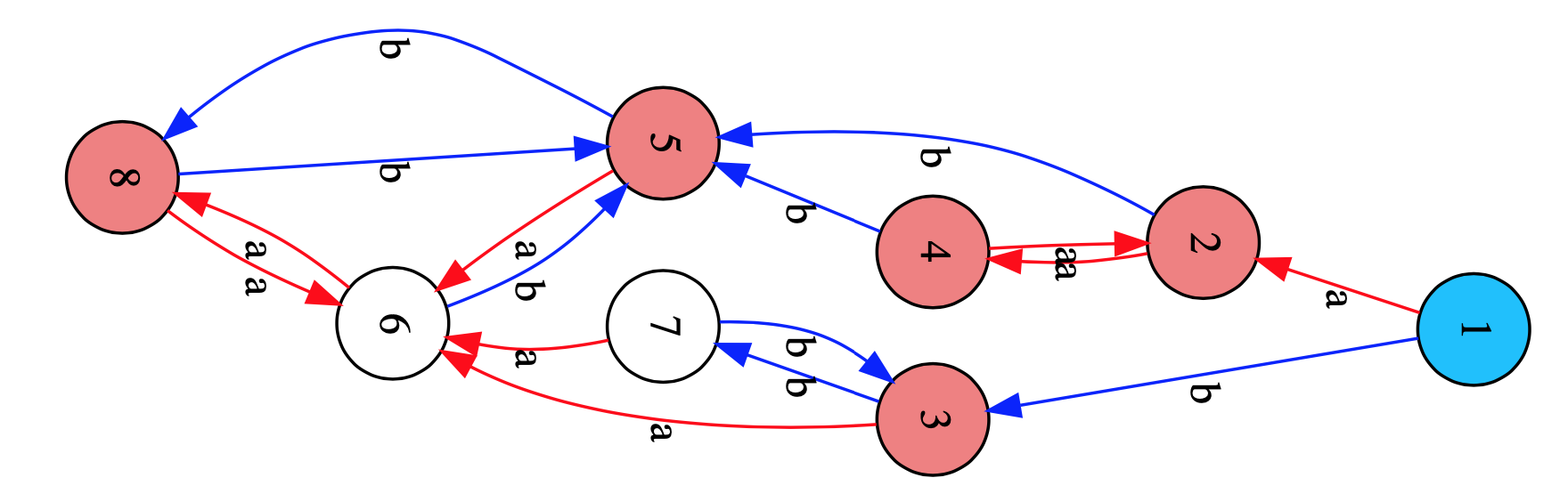
The elements of $T$ (vertices) which can be connected by oriented paths (in both ways) in the Cayley graph, such as here $\{ 2,4 \}$, $\{ 3,7 \}$ and $\{ 5,6,8 \}$, will generate the same right ideal in $T$, so distinct right ideals are determined by unidirectional arrows, such as from $1$ to $2$ and $3$ or from $\{ 2,4 \}$ to $5$, or from $\{ 3,7 \}$ to $6$.

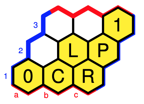
This gives us that $\Omega$ consists of the following six elements:

• $0 = \emptyset$
• $C = \{ 5,6,8 \} = a.T \wedge b.T$
• $L = \{ 2,4,5,6,8 \}=a.T$
• $R = \{ 3,7,5,6,8 \}=b.T$
• $P = \{ 2,3,4,5,6,7,8 \}=a.T \vee b.T$
• $1 = T$

As a subobject classifier $\Omega$ is itself a presheaf, so wat is the action of the triad monoid $T$ on it? For all $A \in \Omega$, and $s \in T$ the action is given by $A.s = \{ t \in T | s.t \in A \}$ and it can be read off from the Cayley-graph.

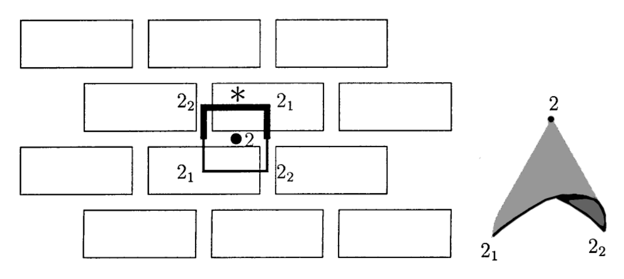
$\Omega$ is a Heyting algebra of which the inclusions, and logical operations can be summarised in the picture below, using the Hexboards and Heytings-post.

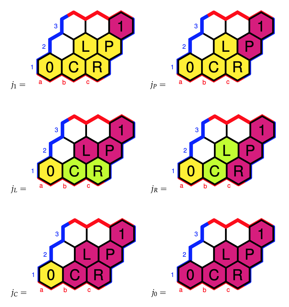
In this case, Grothendieck topologies coincide with Lawvere-Tierney topologies, which come from closure operators $j~:~\Omega \rightarrow \Omega$ which are order-increasing, idempotent, and compatible with the $T$-action and with the $\wedge$, that is,

• if $A \leq B$, then $j(A) \leq j(B)$
• $j(j(A)) = j(A)$
• $j(A).t=j(A.t)$
• $j(A \wedge B) = j(A) \wedge j(B)$

Colouring all cells with the same $j$-value alike, and remaining cells $A$ with $j(A)=A$ coloured yellow, we have six such closure operations $j$, that is, Grothendieck topologies.

The triadic monoid $T$ acts via affine transformations on the set of pitch classes $\mathbb{Z}_{12}$ and we’ve defined it such that it preserves the notes $\{ 0,4,7 \}$ of the major $(0,4,7)$-chord, that is, $\{ 0,4,7 \}$ is a subobject of $\mathbb{Z}_{12}$ in the topos of $T$-sets.

The point of the subobject classifier $\Omega$ is that morphisms to it classify subobjects, so there must be a $T$-equivariant map $\chi$ making the diagram commute (vertical arrows are the natural inclusions)
\[
\xymatrix{\{ 0,4,7 \} \ar[r] \ar[d] & 1 \ar[d] \\ \mathbb{Z}_{12} \ar[r]^{\chi} & \Omega} \]

What does the morphism $\chi$ do on the other pitch classes? Well, it send an element $k \in \mathbb{Z}_{12} = \{ 1,2,\dots,12=0 \}$ to

• $1$ iff $k \in \{ 0,4,7 \}$
• $P$ iff $a(k)$ and $b(k)$ are in $\{ 0,4,7 \}$
• $L$ iff $a(k) \in \{ 0,4,7 \}$ but $b(k)$ is not
• $R$ iff $b(k) \in \{ 0,4,7 \}$ but $a(k)$ is not
• $C$ iff neither $a(k)$ nor $b(k)$ is in $\{ 0,4,7 \}$

Remember that $a$ and $b$ are the transformations (images of $(1,2,\dots,12)$)

a:=Transformation([10,1,4,7,10,1,4,7,10,1,4,7]);;
b:=Transformation([12,8,4,12,8,4,12,8,4,12,8,4]);;

so we see that

• $0,1,4$ are mapped to $1$
• $3$ is mapped to $P$
• $8,11$ are mapped to $L$
• $1,6,9,10$ are mapped to $R$
• $2,5$ are mapped to $C$

Finally, we can compute the sheafification of the sub-presheaf $\{ 0,4,7 \}$ of $\mathbb{Z}$ with respect to a Grothendieck topology $j$: it consists of the set of those $k \in \mathbb{Z}_{12}$ such that $j(\chi(k)) = 1$.

The musically interesting Grothendieck topologies are $j_P, j_L$ and $j_R$ with corresponding sheaves:

• For $j_P$ we get the sheaf $\{ 0,3,4,7 \}$ which Mamuth-ers call a Major-Minor Mixture as these are the notes of both the major and minor $0$-triads
• For $j_L$ we get $\{ 0,3,4,7,8,11 \}$ which is an example of an Hexatonic scale (six notes), here they are the notes of the major and minor $0,~4$ and $8$-triads
• For $j_R$ we get $\{ 0,1,3,4,6,7,9,10 \}$ which is an example of an Octatonic scale (eight notes), here they are the notes of the major and minor $0,~3,~6$ and $9$-triads

We could have played the same game starting with the three notes of any other major triad.

Those in the know will have noticed that so far I’ve avoided another incarnation of the dihedral $D_{12}$ group in music, namely the $PLR$-group, which explains the notation for the elements of the subobject classifier $\Omega$, but this post is already way too long.

(to be continued…)

Leave a Comment