Last time, we’ve seen that the first time ‘schemes’ were introduced was in ‘La Tribu’ (the internal Bourbaki-account of their congresses) of the May-June 1955 congress in Chicago.
Here, we will focus on the events leading up to that event. If you always thought Grothendieck invented the word ‘schemes’, here’s what Colin McLarty wrote:
“A story says that in a Paris café around 1955 Grothendieck asked his friends “what is a scheme?”. At the time only an undefined idea of “schéma” was current in Paris, meaning more or less whatever would improve on Weil’s foundations.” (McLarty in The Rising Sea)
What were Weil’s foundations of algebraic geometry?
Well, let’s see how Weil defined an affine variety over a field $k$. First you consider a ‘universal field’ $K$ containing $k$, that is, $K$ is an algebraically closed field of infinite transcendence degree over $k$. A point of $n$-dimensional affine space is an $n$-tuple $x=(x_1,\dots,x_n) \in K^n$. For such a point $x$ you consider the field $k(x)$ which is the subfield of $K$ generated by $k$ and the coordinates $x_i$ of $x$.
Alternatively, the field $k(x)$ is the field of fractions of the affine domain $R=k[z_1,\dots,z_n]/I$ where $I$ is the prime ideal of all polynomials $f \in k[z_1,\dots,z_n]$ such that $f(x) = f(x_1,\dots,x_n)=0$.
An affine $k$-variety $V$ is associated to a ‘generic point’ $x=(x_1,\dots,x_n)$, meaning that the field $k(x)$ is a ‘regular extension’ of $k$ (that is, for all field-extensions $k’$ of $k$, the tensor product $k(x) \otimes_k k’$ does not contain zero-divisors.
The points of $V$ are the ‘specialisations’ of $x$, that is, all points $y=(y_1,\dots,y_n)$ such that $f(y_1,\dots,y_n)=0$ for all $f \in I$.
Perhaps an example? Let $k = \mathbb{Q}$ and $K=\mathbb{C}$ and take $x=(i,\pi)$ in the affine plane $\mathbb{C}^2$. What is the corresponding prime ideal $I$ of $\mathbb{Q}[z_1,z_2]$? Well, $i$ is a solution to $z_1^2+1=0$ whereas $\pi$ is transcendental over $\mathbb{Q}$, so $I=(z_1^2+1)$ and $R=\mathbb{Q}[z_1,z_2]/I= \mathbb{Q}(i)[z_2]$.
Is $x=(i,\pi)$ a generic point? Well, suppose it were, then the points of the corresponding affine variety $V$ would be all couples $(\pm i, \lambda)$ with $\lambda \in \mathbb{C}$ which is the union of two lines in $\mathbb{C}^2$. But then $i \otimes 1 + 1 \otimes i$ is a zero-divisor in $\mathbb{Q}(x) \otimes_{\mathbb{Q}} \mathbb{Q}(i)$. So no, it is not a generic point over $\mathbb{Q}$ and does not define an affine $\mathbb{Q}$-variety.
If we would have started with $k=\mathbb{Q}(i)$, then $x=(i,\pi)$ is generic and the corresponding affine variety $V$ consists of all points $(i,\lambda) \in \mathbb{C}^2$.
If this is new to you, consider yourself lucky to be young enough to have learned AG from Fulton’s Algebraic curves, or Hartshorne’s chapter 1 if you were that ambitious.
By 1955, Serre had written his FAC, and Bourbaki had developed enough commutative algebra to turn His attention to algebraic geometry.
La Ciotat congress (February 27th – March 6th, 1955)
With a splendid view on the mediterranean, a small group of Bourbaki members (Henri Cartan (then 51), with two of his former Ph.D. students: Jean-Louis Koszul (then 34), and Jean-Pierre Serre (then 29, and fresh Fields medaillist), Jacques Dixmier (then 31), and Pierre Samuel (then 34), a former student of Zariski’s) discussed a previous ‘Rapport de Geometrie Algebrique'(no. 206) and arrived at some unanimous decisions:
1. Algebraic varieties must be sets of points, which will not change at every moment.
2. One should include ‘abstract’ varieties, obtained by gluing (fibres, etc.).
3. All necessary algebra must have been previously proved.
4. The main application of purely algebraic methods being characteristic p, we will hide nothing of the unpleasant phenomena that occur there.

(Henri Cartan and Jean-Pierre Serre, photo by Paul Halmos)
The approach the propose is clearly based on Serre’s FAC. The points of an affine variety are the maximal ideals of an affine $k$-algebra, this set is equipped with the Zariski topology such that the local rings form a structure sheaf. Abstract varieties are then constructed by gluing these topological spaces and sheaves.
At the insistence of the ‘specialistes’ (Serre, and Samuel who had just written his book ‘Méthodes d’algèbre abstraite en géométrie algébrique’) two additional points are adopted, but with some hesitation. The first being a jibe at Weil:
1. …The congress, being a little disgusted by the artificiality of the generic point, does not want $K$ to be always of infinite transcendent degree over $k$. It admits that generic points are convenient in certain circumstances, but refuses to see them put to all the sauces: one could speak of a coordinate ring or of a functionfield without stuffing it by force into $K$.
2. Trying to include the arithmetic case.
The last point was problematic as all their algebras were supposed to be affine over a field $k$, and they wouldn’t go further than to allow the overfield $K$ to be its algebraic closure. Further, (and this caused a lot of heavy discussions at coming congresses) they allowed their varieties to be reducible.
The Chicago congress (May 30th – June 2nd 1955)
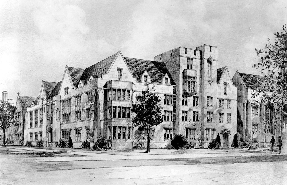
Apart from Samuel, a different group of Bourbakis gathered for the ‘second Caucus des Illinois’ at Eckhart Hall, including three founding members Weil (then 49), Dixmier (then 49) and Chevalley (then 46), and two youngsters, Armand Borel (then 32) and Serge Lang (then 28).
Their reaction to the La Ciotat meeting (the ‘congress of the public bench’) was swift:
(page 1) : “The caucus discovered a public bench near Eckhart Hall, but didn’t do much with it.”
(page 2) : “The caucus did not judge La Ciotat’s plan beyond reproach, and proposed a completely different plan.”
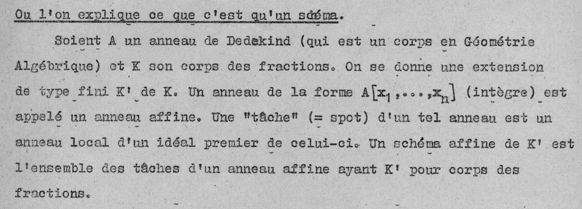
They wanted to include the arithmetic case by defining as affine scheme the set of all prime ideals (or rather, the localisations at these prime ideals) of a finitely generated domain over a Dedekind domain. They continue:
(page 4) : “The notion of a scheme covers the arithmetic case, and is extracted from the illustrious works of Nagata, themselves inspired by the scholarly cogitations of Chevalley. This means that the latter managed to sell all his ideas to the caucus. The Pope of Chicago, very happy to be able to reject very far projective varieties and Chow coordinates, willingly rallied to the suggestions of his illustrious colleague. However, we have not attempted to define varieties in the arithmetic case. Weil’s principle is that it is unclear what will come out of Nagata’s tricks, and that the only stable thing in arithmetic theory is reduction modulo $p$ a la Shimura.”
“Contrary to the decisions of La Ciotat, we do not want to glue reducible stuff, nor call them varieties. … We even decide to limit ourselves to absolutely irreducible varieties, which alone will have the right to the name of varieties.”
The insistence on absolutely irreducibility is understandable from Weil’s perspective as only they will have a generic point. But why does he go along with Chevalley’s proposal of an affine scheme?
In Weil’s approach, a point of the affine variety $V$ determined by a generic point $x=(x_1,\dots,x_n)$ determines a prime ideal $Q$ of the domain $R=k[x_1,\dots,x_n]$, so Chevalley’s proposal to consider all prime ideals (rather than only the maximal ideals of an affine algebra) seems right to Weil.
However in Weil’s approach there are usually several points corresponding to the same prime ideal $Q$ of $R$, namely all possible embeddings of the ring $R/Q$ in that huge field $K$, so whenever $R/Q$ is not algebraic over $k$, there are infinitely Weil-points of $V$ corresponding to $Q$ (whence the La Ciotat criticism that points of a variety were not supposed to change at every moment).
According to Ralf Krömer in his book Tool and Object – a history and philosophy of category theory this shift from Weil-points to prime ideals of $R$ may explain Chevalley’s use of the word ‘scheme’:
(page 164) : “The ‘scheme of the variety’ denotes ‘what is invariant in a variety’.”
Another time we will see how internal discussion influenced the further Bourbaki congresses until Grothendieck came up with his ‘hyperplan’.
Leave a Comment