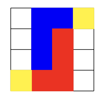
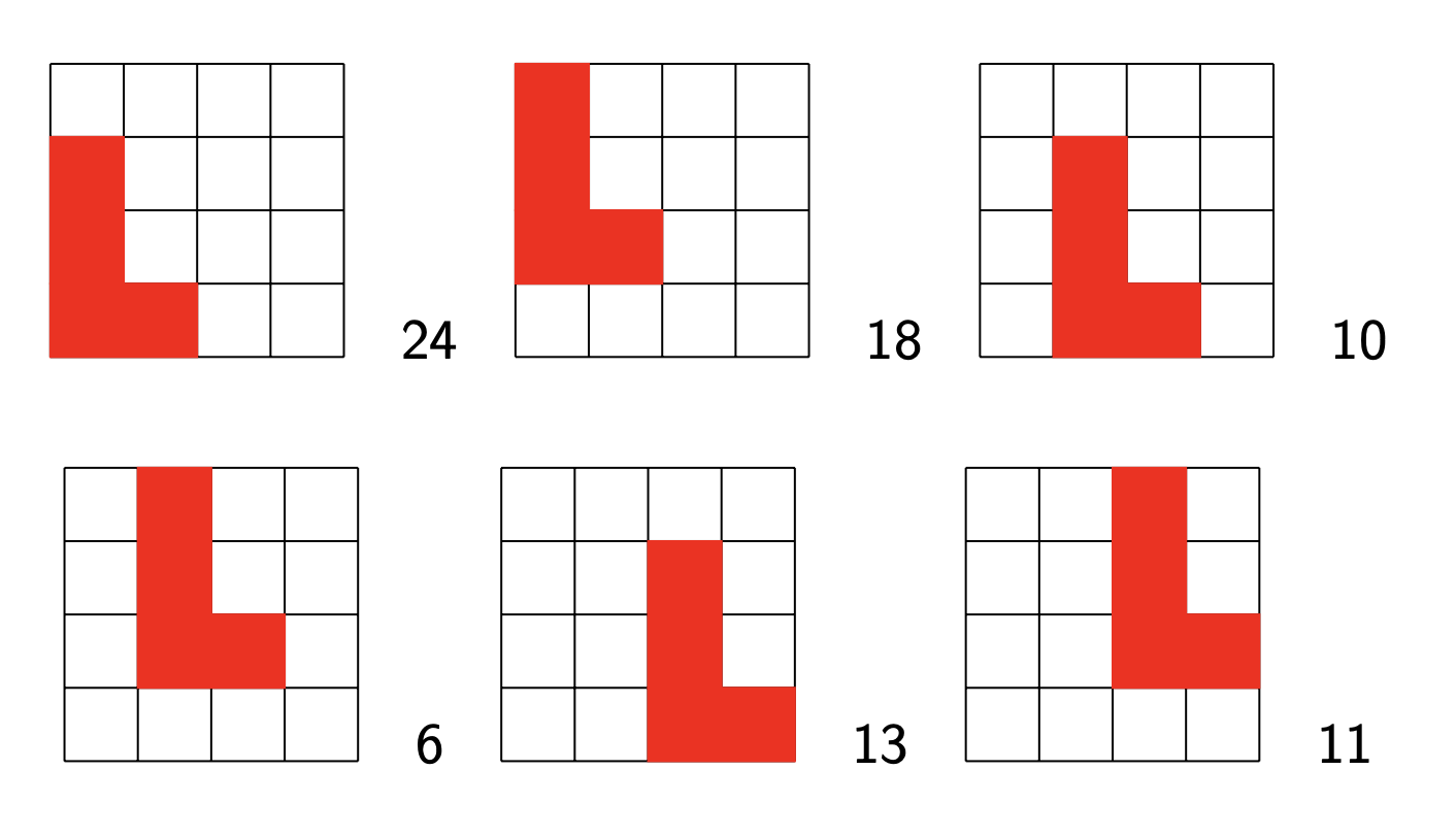
Last time, we’ve viewed major and minor triads (chords) as inscribed triangles in a regular $12$-gon.
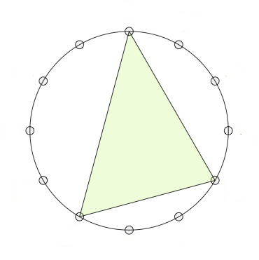
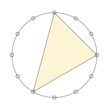
If we move clockwise along the $12$-gon, starting from the endpoint of the longest edge (the root of the chord, here the $0$-vertex) the edges skip $3,2$ and $4$ vertices (for a major chord, here on the left the major $0$-chord) or $2,3$ and $4$ vertices (for a minor chord, here on the right the minor $0$-chord).
The symmetries of the $12$-gon, the dihedral group $D_{12}$, act on the $24$ major- and minor-chords transitively, preserving the type for rotations, and interchanging majors with minors for reflections.
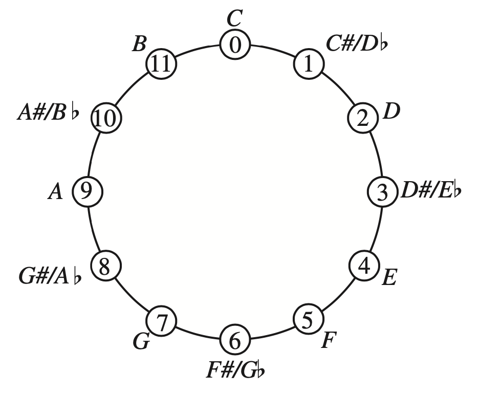
Mathematical Music Theoreticians (MaMuTh-ers for short) call this the $T/I$-group, and view the rotations of the $12$-gon as transpositions $T_k : x \mapsto x+k~\text{mod}~12$, and the reflections as involutions $I_k : x \mapsto -x+k~\text{mod}~12$.
Note that the elements of the $T/I$-group act on the vertices of the $12$-gon, from which the action on the chord-triangles follows.
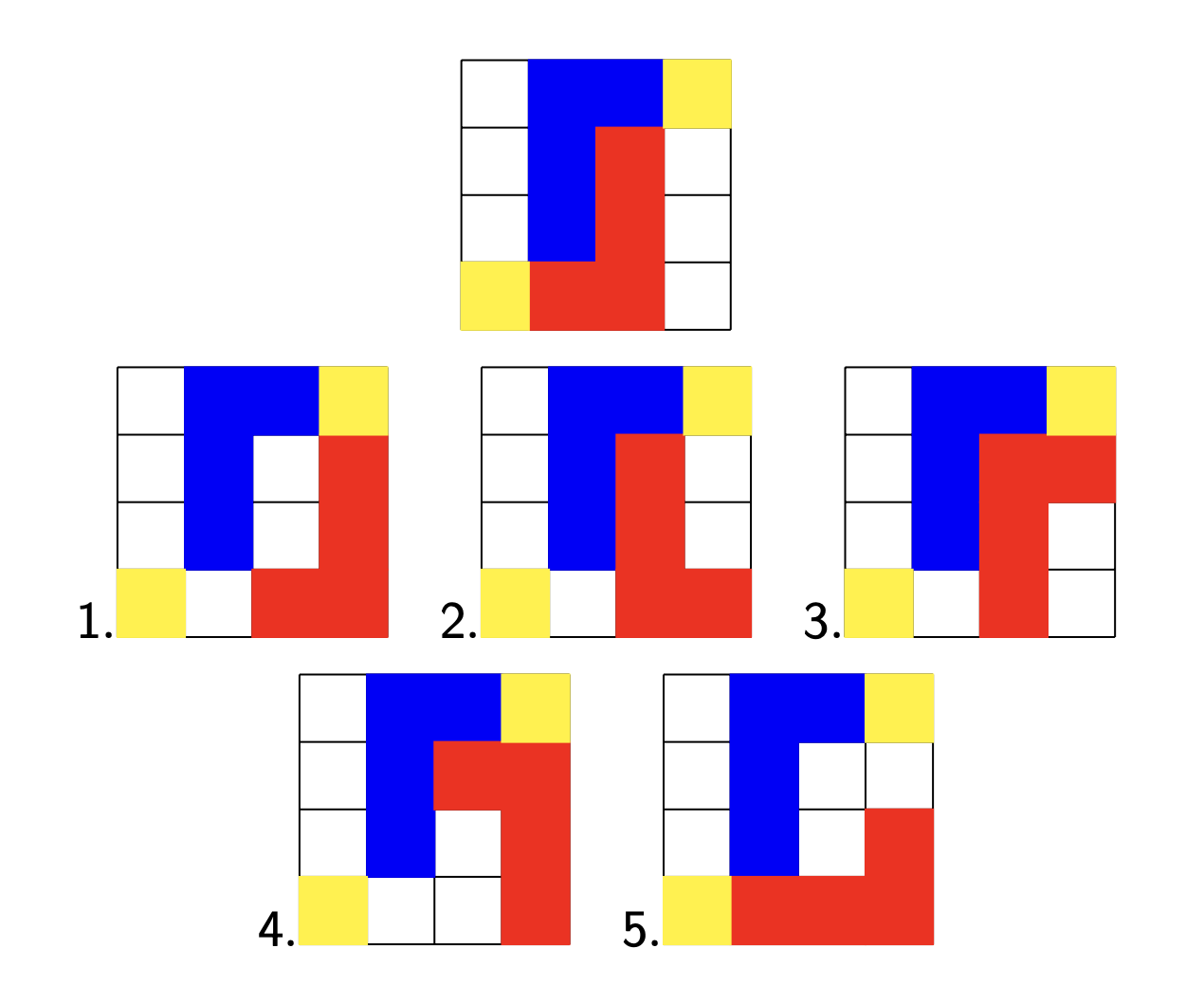
There is another action on the $24$ major and minor chords, mapping a chord-triangle to its image under a reflection in one of its three sides.
Note that in this case the reflection $I_k$ used will depend on the root of the chord, so this action on the chords does not come from an action on the vertices of the $12$-gon.
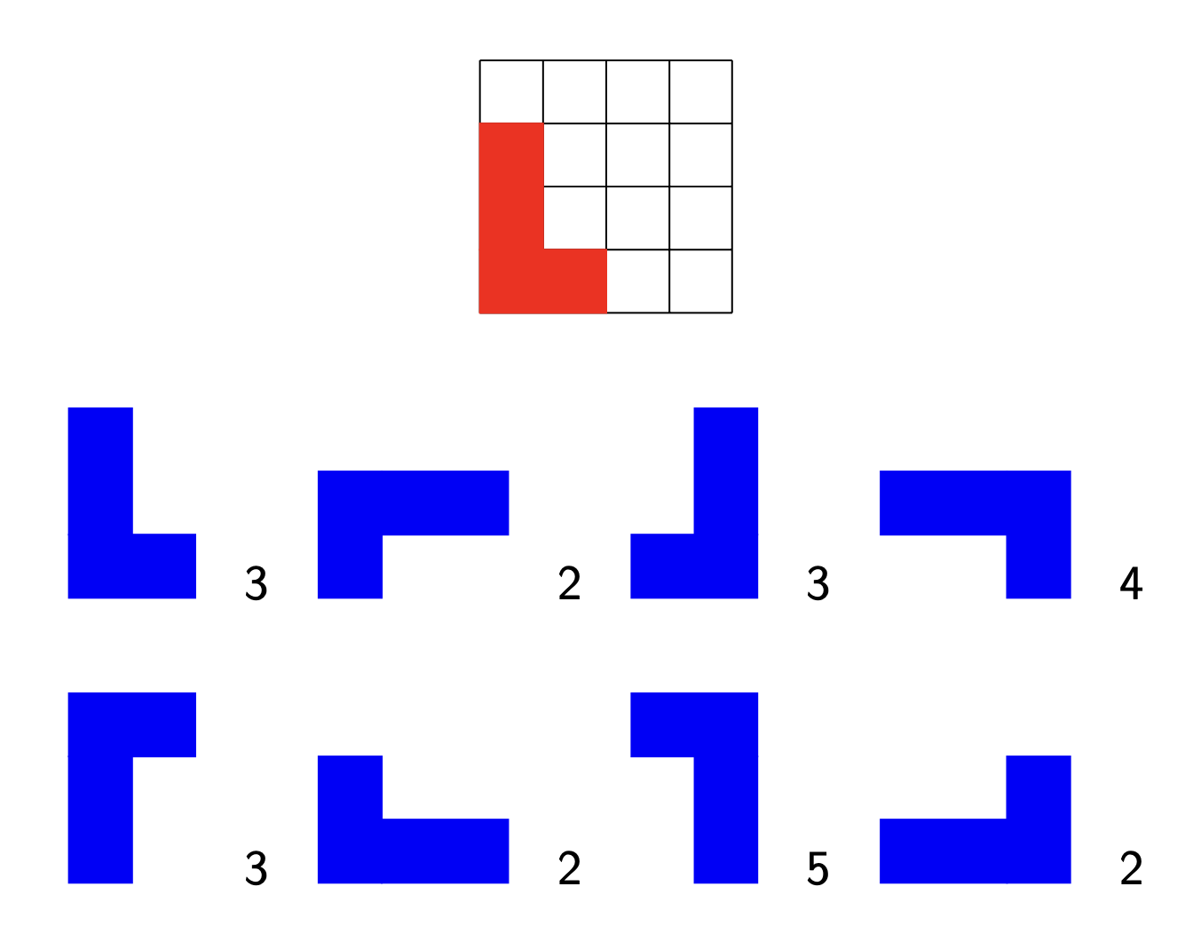
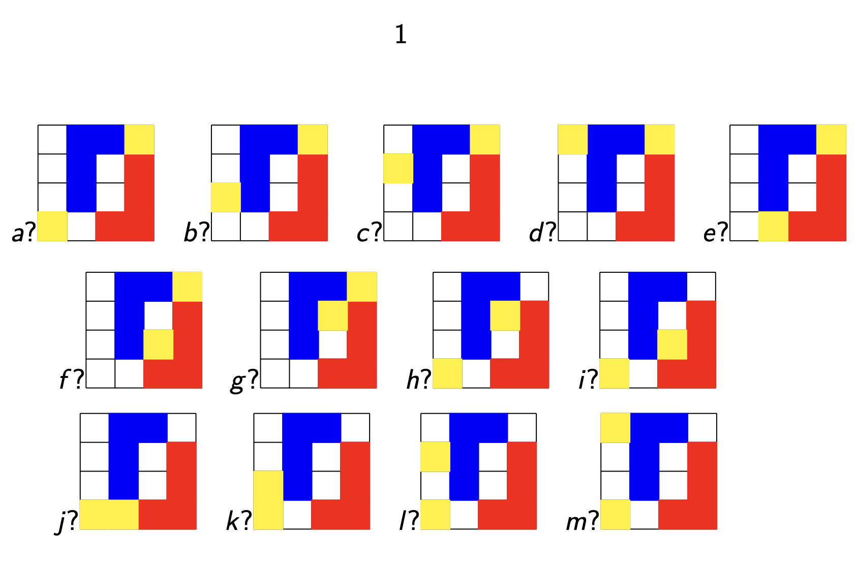
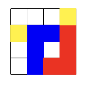
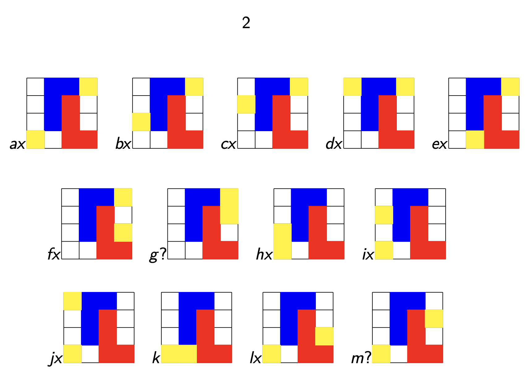
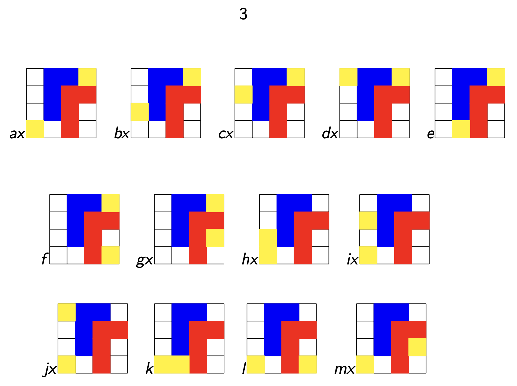
There are three such operations: (pictures are taken from Alexandre Popoff’s blog, with the ‘funny names’ removed)
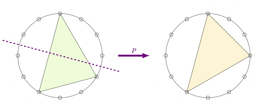
The $P$-operation is reflection in the longest side of the chord-triangle. As the longest side is preserved, $P$ interchanges the major and minor chord with the same root.
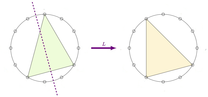
The $L$-operation is refection in the shortest side. This operation interchanges a major $k$-chord with a minor $k+4~\text{mod}~12$-chord.
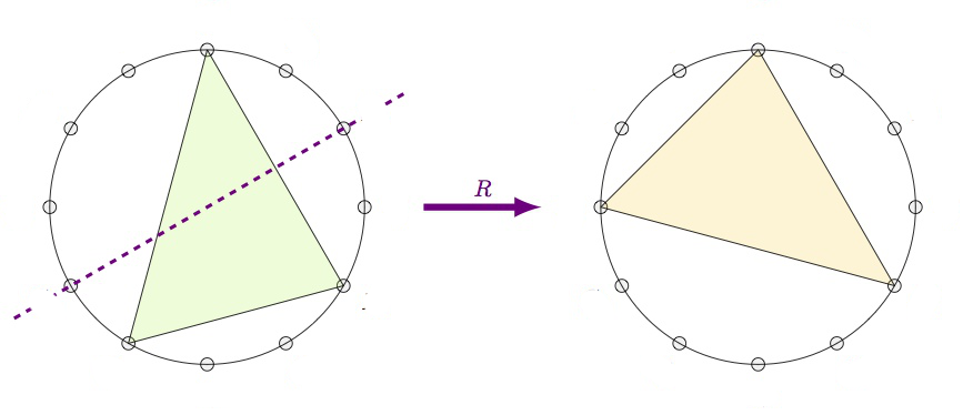
Finally, the $R$-operation is reflection in the middle side. This operation interchanges a major $k$-chord with a minor $k+9~\text{mod}~12$-chord.
From this it is already clear that the group generated by $P$, $L$ and $R$ acts transitively on the $24$ major and minor chords, but what is this $PLR$-group?
If we label the major chords by their root-vertex $1,2,\dots,12$ (GAP doesn’t like zeroes), and the corresponding minor chords $13,14,\dots,24$, then these operations give these permutations on the $24$ chords:
P:=(1,13)(2,14)(3,15)(4,16)(5,17)(6,18)(7,19)(8,20)(9,21)(10,22)(11,23)(12,24)

L:=(1,17)(2,18)(3,19)(4,20)(5,21)(6,22)(7,23)(8,24)(9,13)(10,14)(11,15)(12,16)

R:=(1,22)(2,23)(3,24)(4,13)(5,14)(6,15)(7,16)(8,17)(9,18)(10,19)(11,20)(12,21)
Then GAP gives us that the $PLR$-group is again isomorphic to $D_{12}$:
gap> G:=Group(P,L,R);;

gap> Size(G);

24

gap> IsDihedralGroup(G);

true
In fact, if we view both the $T/I$-group and the $PLR$-group as subgroups of the symmetric group $Sym(24)$ via their actions on the $24$ major and minor chords, these groups are each other centralizers! That is, the $T/I$-group and $PLR$-group are dual to each other.
For more on this, there’s a beautiful paper by Alissa Crans, Thomas Fiore and Ramon Satyendra: Musical Actions of Dihedral Groups.
What does this new MaMuTh info learns us more about our Elephant, the Topos of Triads, studied by Thomas Noll?
Last time we’ve seen the eight element triadic monoid $T$ of all affine maps preserving the three tones $\{ 0,4,7 \}$ of the major $0$-chord, computed the subobject classified $\Omega$ of the corresponding topos of presheaves, and determined all its six Grothendieck topologies, among which were these three:
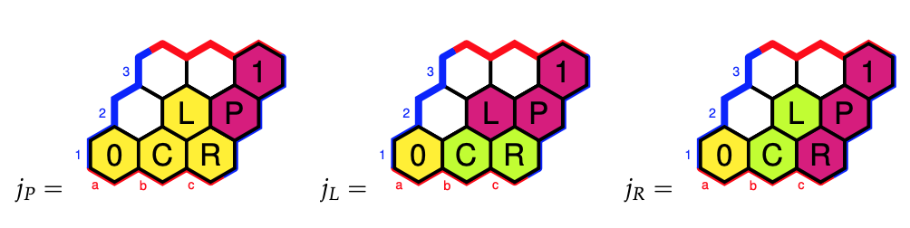
Why did we label these Grothendieck topologies (and corresponding elements of $\Omega$) by $P$, $L$ and $R$?
We’ve seen that the sheafification of the presheaf $\{ 0,4,7 \}$ in the triadic topos under the Grothendieck topology $j_P$ gave us the sheaf $\{ 0,3,4,7 \}$, and these are the tones of the major $0$-chord together with those of the minor $0$-chord, that is the two chords in the $\langle P \rangle$-orbit of the major $0$-chord. The group $\langle P \rangle$ is the cyclic group $C_2$.
For the sheafication with respect to $j_L$ we found the $T$-set $\{ 0,3,4,7,8,11 \}$ which are the tones of the major and minor $0$-,$4$-, and $8$-chords. Again, these are exactly the six chords in the $\langle P,L \rangle$-orbit of the major $0$-chord. The group $\langle P,L \rangle$ is isomorphic to $Sym(3)$.
The $j_R$-topology gave us the $T$-set $\{ 0,1,3,4,6,7,9,10 \}$ which are the tones of the major and minor $0$-,$3$-, $6$-, and $9$-chords, and lo and behold, these are the eight chords in the $\langle P,R \rangle$-orbit of the major $0$-chord. The group $\langle P,R \rangle$ is the dihedral group $D_4$.
More on this can be found in the paper Commuting Groups and the Topos of Triads by Thomas Fiore and Thomas Noll.
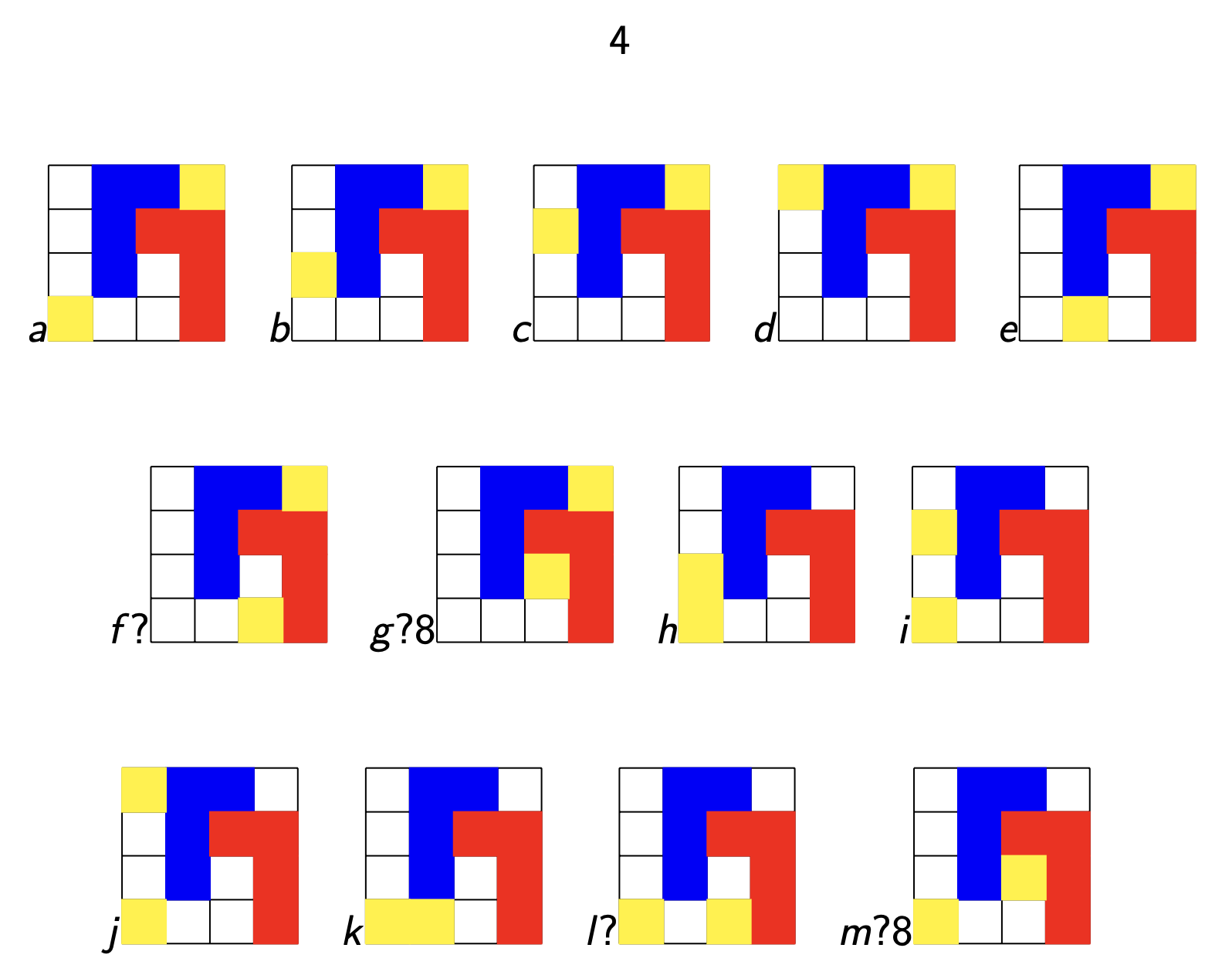
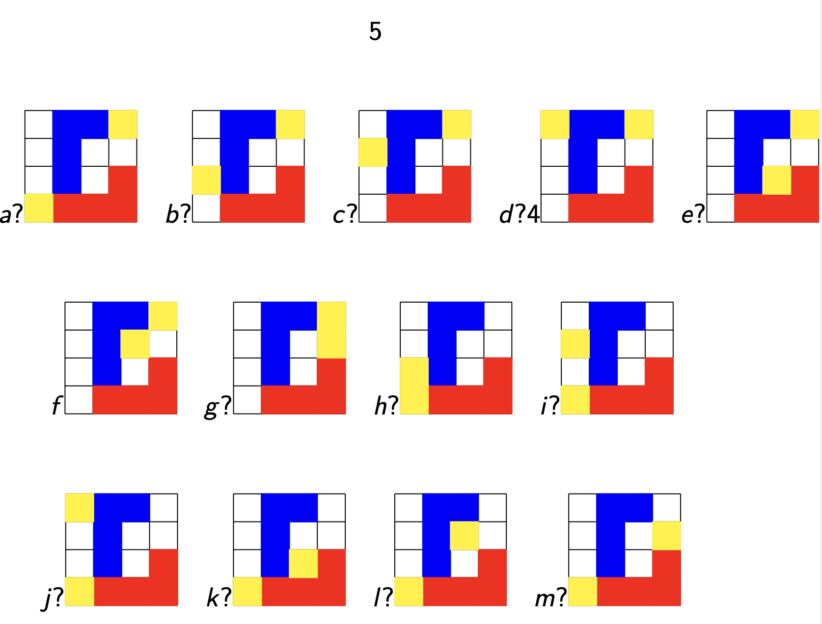
The operations $P$, $L$ and $R$ on major and minor chords are reflexions in one side of the chord-triangle, so they preserve two of the three tones. There’s a distinction between the $P$ and $L$ operations and $R$ when it comes to how the third tone changes.
Under $P$ and $L$ the third tone changes by one halftone (because the corresponding sides skip an even number of vertices), whereas under $R$ the third tone changes by two halftones (a full tone), see the pictures above.
The $\langle P,L \rangle = Sym(3)$ subgroup divides the $24$ chords in four orbits of six chords each, three major chords and their corresponding minor chords. These orbits consist of the
- $0$-, $4$-, and $8$-chords (see before)
- $1$-, $5$-, and $9$-chords
- $2$-, $6$-, and $10$-chords
- $3$-, $7$-, and $11$-chords
and we can view each of these orbits as a cycle tracing six of the eight vertices of a cube with one pair of antipodal points removed.
These four ‘almost’ cubes are the NE-, SE-, SW-, and NW-regions of the Cube Dance Graph, from the paper Parsimonious Graphs by Jack Douthett and Peter Steinbach.
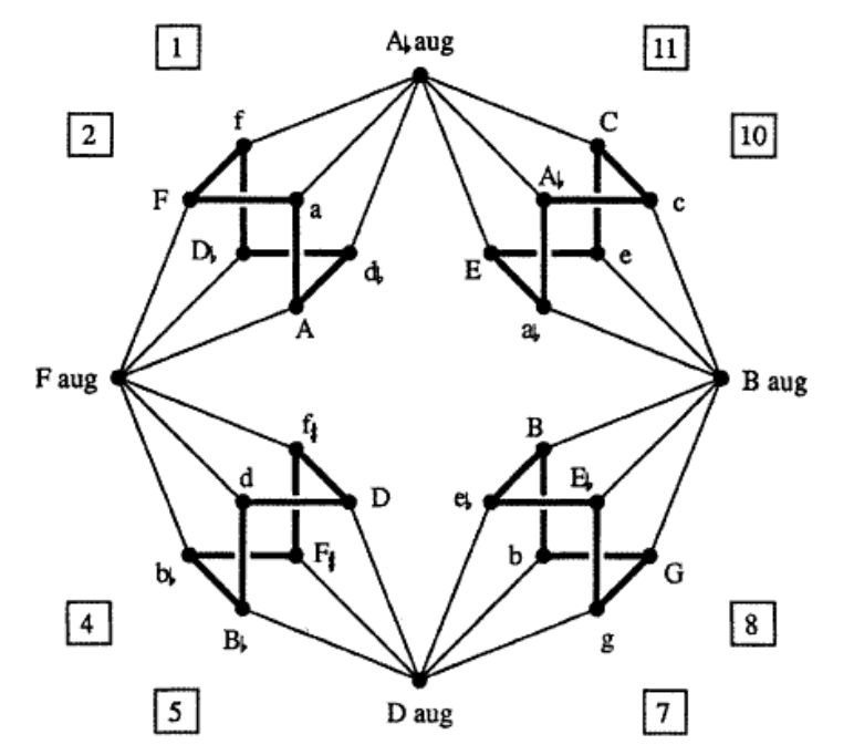
To translate the funny names to our numbers, use this dictionary (major chords are given by a capital letter):
The four extra chords (at the N, E, S, and P places) are augmented triads. They correspond to the triads $(0,4,8),~(1,5,9),~(2,6,10)$ and $(3,7,11)$.
That is, two triads are connected by an edge in the Cube Dance graph if they share two tones and differ by an halftone in the third tone.
This graph screams for a group or monoid acting on it. Some of the edges we’ve already identified as the action of $P$ and $L$ on the $24$ major and minor triads. Because the triangle of an augmented triad is equilateral, we see that they are preserved under $P$ and $L$.
But what about the edges connecting the regular triads to the augmented ones? If we view each edge as two directed arrows assigned to the same operation, we cannot do this with a transformation because the operation sends each augmented triad to six regular triads.
Alexandre Popoff, Moreno Andreatta and Andree Ehresmann suggest in their paper Relational poly-Klumpenhouwer networks for transformational and voice-leading analysis that one might use a monoid generated by relations, and they show that there is such a monoid with $40$ elements acting on the Cube Dance graph.
Popoff claims that usual presheaf toposes, that is contravariant functors to $\mathbf{Sets}$ are not enough to study transformational music theory. He suggest to use instead functors to $\mathbf{Rel}$, that is Sets with as the morphisms binary relations, and their compositions.
Another Elephant enters the room…
(to be continued)