Monstrous moonshine was born (sometime in 1978) the moment John McKay realized that the linear term in the j-function
$j(q) = \frac{1}{q} + 744 + 196884 q + 21493760 q^2 + 864229970 q^3 + \ldots $
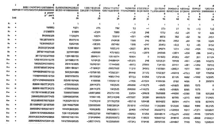
is surprisingly close to the dimension of the smallest non-trivial irreducible representation of the monster group, which is 196883. Note that at that time, the Monster hasn’t been constructed yet, and, the only traces of its possible existence were kept as semi-secret information in a huge ledger (costing 80 pounds…) kept in the Atlas-office at Cambridge. Included were 8 huge pages describing the character table of the monster, the top left fragment, describing the lower dimensional irreducibles and their characters at small order elements, reproduced below
If you look at the dimensions of the smallest irreducible representations (the first column) : 196883, 21296876, 842609326, … you will see that the first, second and third of them are extremely close to the linear, quadratic and cubic coefficient of the j-function. In fact, more is true : one can obtain these actual j-coefficients as simple linear combination of the dimensions of the irrducibles :
$\begin{cases} 196884 &= 1 + 196883 \\
21493760 &= 1 + 196883 + 21296876 \\
864229970 &= 2 \times 1 + 2 \times 196883 + 21296876 + 842609326
\end{cases} $
Often, only the first relation is attributed to McKay, whereas the second and third were supposedly discovered by John Thompson after MKay showed him the first. Marcus du Sautoy tells a somewhat different sory in Finding Moonshine :
McKay has also gone on to find these extra equations, but is was Thompson who first published them. McKay admits that “I was a bit peeved really, I don’t think Thompson quite knew how much I knew.”
By the work of Richard Borcherds we now know the (partial according to some) explanation behind these numerical facts : there is a graded representation $V = \oplus_i V_i $ of the Monster-group (actually, it has a lot of extra structure such as being a vertex algebra) such that the dimension of the i-th factor $V_i $ equals the coefficient f $q^i $ in the j-function. The homogeneous components $V_i $ being finite dimensional representations of the monster, they decompose into the 194 irreducibles $X_j $. For the first three components we have the decompositions
$\begin{cases} V_1 &= X_1 \oplus X_2 \\
V_2 &= X_1 \oplus X_2 \oplus X_3 \\
V_3 &= X_1^{\oplus 2 } \oplus X_2^{\oplus 2} \oplus X_3 \oplus X_4
\end{cases} $
Calculating the dimensions on both sides give the above equations. However, being isomorphisms of monster-representations we are not restricted to just computing the dimensions. We might as well compute the character of any monster-element on both sides (observe that the dimension is just the character of the identity element). Characters are the traces of the matrices describing the action of a monster-element on the representation and these numbers fill the different columns of the character-table above.
Hence, the same integral combinations of the character values of any monster-element give another q-series and these are called the McKay-Thompson series. John Conway discovered them to be classical modular functions known as Hauptmoduln.
In most papers and online material on this only the first few coefficients of these series are documented, which may be just too little information to make new discoveries!
Fortunately, David Madore has compiled the first 3200 coefficients of all the 172 monster-series which are available in a huge 8Mb file. And, if you really need to have more coefficients, you can always use and modify his moonshine python program.
In order to reduce bandwidth, here a list containing the first 100 coefficients of the j-function
jfunct=[196884, 21493760, 864299970, 20245856256, 333202640600, 4252023300096, 44656994071935, 401490886656000, 3176440229784420, 22567393309593600, 146211911499519294, 874313719685775360, 4872010111798142520, 25497827389410525184, 126142916465781843075, 593121772421445058560, 2662842413150775245160, 11459912788444786513920, 47438786801234168813250, 189449976248893390028800, 731811377318137519245696, 2740630712513624654929920, 9971041659937182693533820, 35307453186561427099877376, 121883284330422510433351500, 410789960190307909157638144, 1353563541518646878675077500, 4365689224858876634610401280, 13798375834642999925542288376, 42780782244213262567058227200, 130233693825770295128044873221, 389608006170995911894300098560, 1146329398900810637779611090240, 3319627709139267167263679606784, 9468166135702260431646263438600, 26614365825753796268872151875584, 73773169969725069760801792854360, 201768789947228738648580043776000, 544763881751616630123165410477688, 1452689254439362169794355429376000, 3827767751739363485065598331130120, 9970416600217443268739409968824320, 25683334706395406994774011866319670, 65452367731499268312170283695144960, 165078821568186174782496283155142200, 412189630805216773489544457234333696, 1019253515891576791938652011091437835, 2496774105950716692603315123199672320, 6060574415413720999542378222812650932, 14581598453215019997540391326153984000, 34782974253512490652111111930326416268, 82282309236048637946346570669250805760, 193075525467822574167329529658775261720, 449497224123337477155078537760754122752, 1038483010587949794068925153685932435825, 2381407585309922413499951812839633584128, 5421449889876564723000378957979772088000, 12255365475040820661535516233050165760000, 27513411092859486460692553086168714659374, 61354289505303613617069338272284858777600, 135925092428365503809701809166616289474168, 299210983800076883665074958854523331870720, 654553043491650303064385476041569995365270, 1423197635972716062310802114654243653681152, 3076095473477196763039615540128479523917200, 6610091773782871627445909215080641586954240, 14123583372861184908287080245891873213544410, 30010041497911129625894110839466234009518080, 63419842535335416307760114920603619461313664, 133312625293210235328551896736236879235481600, 278775024890624328476718493296348769305198947, 579989466306862709777897124287027028934656000, 1200647685924154079965706763561795395948173320, 2473342981183106509136265613239678864092991488, 5070711930898997080570078906280842196519646750, 10346906640850426356226316839259822574115946496, 21015945810275143250691058902482079910086459520, 42493520024686459968969327541404178941239869440, 85539981818424975894053769448098796349808643878, 171444843023856632323050507966626554304633241600, 342155525555189176731983869123583942011978493364, 679986843667214052171954098018582522609944965120, 1345823847068981684952596216882155845897900827370, 2652886321384703560252232129659440092172381585408, 5208621342520253933693153488396012720448385783600, 10186635497140956830216811207229975611480797601792, 19845946857715387241695878080425504863628738882125, 38518943830283497365369391336243138882250145792000, 74484518929289017811719989832768142076931259410120, 143507172467283453885515222342782991192353207603200, 275501042616789153749080617893836796951133929783496, 527036058053281764188089220041629201191975505756160, 1004730453440939042843898965365412981690307145827840, 1908864098321310302488604739098618405938938477379584, 3614432179304462681879676809120464684975130836205250, 6821306832689380776546629825653465084003418476904448, 12831568450930566237049157191017104861217433634289960, 24060143444937604997591586090380473418086401696839680, 44972195698011806740150818275177754986409472910549646, 83798831110707476912751950384757452703801918339072000]
This information will come in handy when we will organize our Monstrous Easter Egg Race, starting tomorrow at 6 am (GMT)…
Leave a Comment